One of the most fascinating problems of classical physics is the circular, restricted, three-body problem (CR3BP). Not only is this problem full of rich behaviors that are not exhibited in the Kepler problem or in the problem of a single body moving in an external unchanging force, but the applications of the CR3BP are numerous. For example, the trajectory that the James Webb Space Telescope (JWST) moves along around the Sun-Earth/Moon L2 libration point can only be understood within the context of the CR3BP. Many other spacecraft have been found at these Libration Points, including Wind, ACE, SOHO, WMAP, and the soon-to-be-launched Nancy Grace Roman Space Telescope. (Side note: I’ve contributed to all of these missions, often as the flight dynamics lead, and JWST is currently flying the trajectory I designed for it).

In terms of the complexity and hierarchy of dynamics, the CR3BP positions itself at an interesting junction. It is far more complex than the Kepler problem but far simpler than the generic N-body problem making it at least tractable in many areas.

This post will be the first in a series that explores the CR3BP. Here we will establish the equations of motions, explaining along the way, why the word restricted gets attached. We will then show how moving to a rotating frame transforms the problem from being time-dependent (non-autonomous) to time-independent (autonomous). This rotating frame also has the benefit of revealing the existence of a pseudopotential that turns the equations of motion in the rotating frame into a Hamiltonian system (but we will have to wait until a future post to see that). At the end, I’ll comment on what makes the circular case much simpler than the elliptic, restricted, three-body problem.

The argument presented below is highly influenced by Chapter 5 of A E Roy’s book Orbital Motion, 3rd edition.

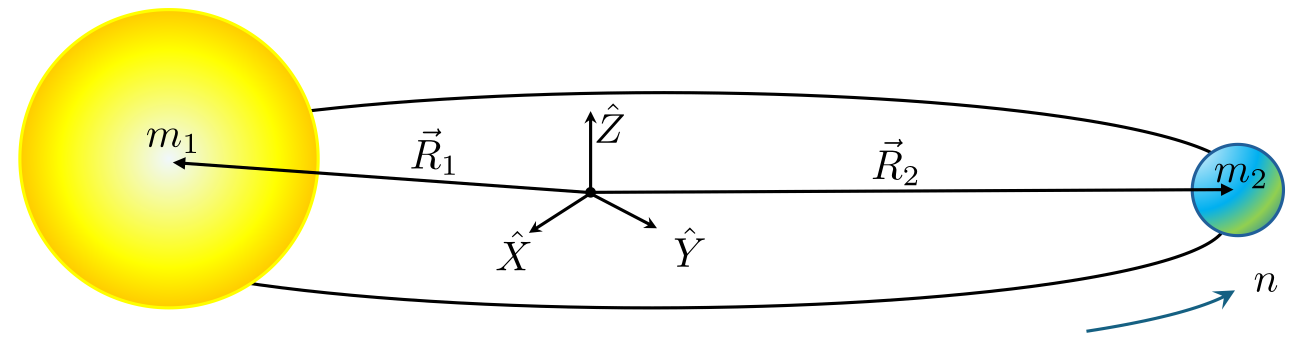
Our study begins with assuming that there are two massive bodies of mass $m_1$ and $m_2$ that are interacting gravitationally with each other. These bodies, referred to as the primary and the secondary, follow motion that is exactly described by the Kepler problem. We layer the additional requirement that the primary and secondary are in circular motion about their center-of-mass with a fixed distance between them of $L$. Under these assumptions, the bodies move at a constant angular rate

\[ n = \sqrt{\frac{G (m_1 + m_2)} {L^3}} \; . \]

Note the use of $n$ (for mean motion) in place of the more traditional elementary symbol $\omega$ for uniform circular motion is to honor the celestial mechanics use. The geometry can be further specified by fixing an inertial coordinate system $\{ {\hat X}, {\hat Y}, {\hat Z} \}$ at the center of mass (with ${\hat X}$ and ${\hat Y}$ in the orbital plane) and by denoting the position vectors of the two bodies with respect to the center of mass as ${\vec R}_1$ and ${\vec R}_2$.

In order to make the treatment universally applicable (e.g., to the Earth-Moon system as well as Sun-Jupiter), units are chosen to make the equations of motion non-dimensional. It is customary in all treatments to pick $L$ as the unit of distance between the masses and the total mass $M = m_1 + m_2$ as the unit of mass. The secondary’s mass is then denoted by the mass fraction parameter $\mu$ (i.e., $m_1 = 1 – \mu$ and $m_2 = \mu$). By its definition $\mu \leq 1/2$. There is no consensus on the choice of the unit of time and there are two reasonable choices: 1) set $G = 1$ so that the angular frequency $n=1$ (i.e., the period of motion is $2 \pi$) or 2) set the unit of time so that the period of motion is unity. We pick option 1) in order to more faithfully follow Roy.

At this point we can introduce the restricted body at a position ${\vec R} = X {\hat X} + Y {\hat Y} + Z {\hat Z}$ and form the equations of motion in the inertial coordinate system (note the mass of the restricted body $m$ plays no role if the forces are solely gravitational)

\[ {\ddot {\vec R}} = – \frac{(1-\mu) ({\vec R}-{\vec R}_1)}{| {\vec R}-{\vec R}_1|^3} – \frac{\mu ({\vec R}-{\vec R}_2)}{| {\vec R}-{\vec R}_2 |^3} \; .\]

While the above equation looks innocent enough, it is worth noting that the force is time-dependent since the primary and secondary execute their motion ignorant of the existence of the restricted body. This point can be driven home if we assume that the line joining the primary to the secondary is aligned with ${\hat X}$ at $t=0$ with the vector pointing to the secondary having a positive value. Their position vectors can be written explicitly as

\[ {\vec R}_1 = -(1-\mu) \left[ \cos t {\hat X} + \sin t {\hat Y} \right] \; \]

and

\[ {\vec R}_2 = \mu \left[ \cos t {\hat X} + \sin t {\hat Y} \right] \; . \]

As a check, one can confirm that at all times $m_1 {\vec R}_1 + m_2 {\vec R}_2 = 0$. Substituting in these expressions transforms the equations of motion (now written in component form] to:

\[ {\ddot X} = -(1-\mu)\frac{X+(1-\mu) \cos t}{D_1^3} + \mu \frac{X-\mu \cos t}{D_2^3} \; , \]

\[ {\ddot Y} = -(1-\mu)\frac{Y+(1-\mu) \sin t}{D_1^3} + \mu \frac{Y-\mu \sin t}{D_2^3} \; , \]

and

\[ {\ddot Z} = -(1-\mu)\frac{Z}{D_1^3} + \mu \frac{Z}{D_2^3} \; . \]

The distances $D_1$ \& $D_2$ between the primary \& secondary and the restricted body, respectively, are given by:

\[ D_1 = \sqrt{ \left[ X + \mu \cos t \right]^2 + \left[ Y + \mu \sin t\right]^2 + Z^2 } \; \]

and

\[ D_2 = \sqrt{ \left[ X – (1-\mu) \cos t \right]^2 + \left[ Y – (1- \mu) \sin t\right]^2 + Z^2 } \; .\]

This form clearly shows that the underlying equations are explicitly time-dependent. Of course, this makes sense since the motion of the restricted particle does not influence the motion of the primary and secondary. Their orbital motion acts like an external force that drives the system but is not part of the system. This is sometimes referred to as the restricted particle reacting to but not ‘back-reacting’ on the other two.

Despite this non-autonomous character, the CR3BP can be cast into a autonomous form. The key insight is to note that since the massive bodies move in circular motion about their center-of-mass, their angular rate is constant.  If we construct a co-rotating frame so that it rotates around ${\hat Z}$ and has it’s x-axis aligned with ${\hat X}$ at $t=0$ then $x_1 = -\mu$ and $x_2 = (1-\mu)$, with $y_1=y_2=z_1=z_2=0$ (with the lower case letters indicating the corresponding components of position measured by an observer moving with this frame). and, so, in a co-rotating frame they will appear fixed. We can relate the position components in the inertial frame with those in this co-rotating frame using

\[ X_i = x_i \cos(t) – y_i \sin(t) \; , \]

\[ Y_i = x_i \sin(t) + y_i \cos(t) \; , \]

and

\[ Z_i = z_i \; . \]

The $i$ index specifies the body in question: restricted $i$ is blank, primary $i=1$, and secondary $i=2$.

We now need to re-express the inertial equations of motion in the co-rotating frame.  We’ll tackle the terms appearing on the left-hand sides first and then right-hand sides second.

The time derivatives of the position components on the left-hand sides are a bit involved since the transformation to the co-rotating frame is time dependent.  Fortunately, only the in-plane components are involved, with the left-hand sides becoming:

\[ LHS_x = {\ddot x} \cos t – 2 {\dot x} \sin t – x \cos t – {\ddot y} \sin t – 2 {\dot y} \cos t + y \sin t \; \]

and

\[ LHS_y = {\ddot y} \cos t – 2 {\dot y} \sin t – y \cos t + {\ddot x} \sin t – 2 {\dot x} \cos t – x \sin t \; .\]

Note that the terms involving a single time derivative (either ${\dot x}$ or ${\dot y}$) appear with opposite signs in the two left-hand sides. This leads to taking linear combinations of the two to isolate the motion for $x$ and $y$, more cleanly:

\[ LHS_x \cos t + LHS_y \sin t = {\ddot x}-2 {\dot y}-x \; \]

and

\[ -LHS_x \sin t + LHS_y \cos t = {\ddot y} + 2{\dot x} – y \; . \]

When we look at the right-hand sides, we see a similar pattern where the in-plane, co-rotating coordinates $x_i$ and $y_i$ mix together when converting each of the independent inertial coordinates.  We can grind through substituting in the transformations above and then combining the right-hand sides in the same way as was done for the left-hand sides above (click here for a Jupyter notebook showing all the steps).  However, there is an easier way that involves more insight but far less industry.  Recognize that since the right-hand side doesn’t depend on time, it can be evaluated completely in the co-rotating frame.  In that frame the position of the restricted body is given by ${\vec R} = x {\hat x} + y {\hat y} + z {\hat z}$ and the specific forces (force/restricted mass) arise as if we hadn’t mixed the equations of motion. 

The distances between the massives and the restricted are:

\[ d_1 = \sqrt{ (x+\mu)^2 + y^2 + z^2 } \; \]

and

\[d_2 = \sqrt{ (x-1+\mu)^2 + y^2 + z^2} \; ,\]

where the switch has been made from upper case ‘D’ to lower case ‘d’ simply to emphasize the difference in structural forms.

\[ {\ddot x} – 2 {\dot y} = x – (1-\mu) \frac{x+\mu}{d_1^3} – \mu \frac{x-1+\mu}{d_2^3} \; , \]

\[ {\ddot y} + 2 {\dot x} = y – (1-\mu) \frac{y}{d_1^3} -\mu \frac{y}{d_2^3} \; , \]

and

\[ {\ddot z} = -(1-\mu) \frac{z}{d_1^3} – \mu \frac{z}{d_2^3} \; ,\]

This final form has successfully eliminated the non-autonomous nature of the inertial equations. This simplification was possible precisely because the co-rotating frame moves with a constant angular rate (i.e., there are no $\dot n$ in the transformation of the left-hand sides). This special case also explains why the difficulty in allowing the primary and secondary to move on elliptical paths is so much more pronounced.

Over the past two installments, we’ve seen that the percolation model, which has at its core simple, static probabilistic rules, exhibits three distinct behaviors.  For the occupation probability $p$ well below the critical probability $p_c$, the lattice is mostly empty with a few isolated islands of filled sites but with extremely little likelihood to have a spanning cluster joining opposites of the lattice.  For the occupation probability well above the critical probability, the lattice is mostly filled and, as a sort of mirror image, the lattice is mostly filled with a few isolated islands of vacant sites and with nearly perfect certainty that a spanning cluster is present.  The third behavior exists in the ‘local’ neighborhood near the critical probability where the observation evidence from computer experiments and the conventional wisdom indicates that many different length sizes exist.

In order to go from that qualitative picture summarized above to a quantitative structure, we need to define the measurements that we can make to the computational lattice.  The most important one is the cluster size distribution $n_s$ defined as the number $n$ of clusters with a size $s$.

The best way to understand $n_s$ is with a few sample lattices.  For the first example, let’s look at a percolation lattice of size $16 \times 16$ with an occupation probability of $p_{occ} = 0.4$. 

**image**

With a bit of patience one might convince oneself that there are 30 distinct clusters.  With a bit more effort, it becomes clear that there 13 distinct clusters with only one site and so we would assign $n_s(1) = 13$.  Likewise, there are 4 distinct clusters of size 2 so that $n_s(2) = 4$, and so on.

The full listing of Cluster ID versus Cluster Size for this lattice is:

note that a cluster with an ID of zero means that the site was not occupied. 

The last post introduced the basic model of site percolation in which an $M \times N$ lattice would have each of its sites occupied with a probability $p$.  It was demonstrated that by sweeping that probability up through a critical value $p_c$ there was a qualitative change in system.  Below $p_c$, there was a small likelihood of finding a spanning cluster, defined as a connected set of sites in which an unbroken path could be made between either the left and right sides of the lattice or the top and bottom of the lattice or both.  Above $p_c$ there it is almost certain that a spanning cluster will exist.  For a cluster to be connected, nearest neighbor sites must be occupied in the up-down direction or the right-left direction.

The percolation model finds itself in the center of a lot of analysis because it is a simple example of a phase transition, in this case what is known as a geometric phase transition.  Phase transitions are familiar in physics and we see numerous examples.  Perhaps the most common place one is $H_2 O$ going from solid form (ice) to liquid (water) to gas (steam).  Percolation provides a simple playground in which the basic ideas and theoretical foundations can be explored without bringing to account the vast machinery of statistical mechanics.   Despite this ‘toy’ status, percolation models are physically interesting in their own way as well.

An enormous amount of work went into understanding how phase transitions occur during the 1960s and 1970s and one of the most celebrated ideas is the notion that the system exhibits a type of length invariance at the transition.  The correlation length, properly defined, becomes infinite, and all length scales matter.

In this entry, I’ll try to show what is meant by this notion before turning, in subsequent columns, to the quantitative theory of critical exponents and scaling laws.  To this end, the results presented here will be more in the line of a numerical experimentalist presenting the findings of a variety of simulations without the presentation of much in the way of an underlying theory to explain the results from a compact set of premises.

These experiments consisted of running 50 trials of the percolation model for each of 4 lattice sizes: $L = 16$, $32$, $64$, and $128$ cells per linear dimension and over five separate occupation probabilities $p = 0.4$, $0.5$, $0.5927 \equiv p_c$, $0.7$, and $0.8$. 

Using the Hoshen-Kopelman cluster identification algorithm, the number of clusters in the lattice were labeled with a unique, sequential cluster id number.  These clusters labels afford the ability to both create visual representations of the lattice and perform quantitative analysis. 

We’ll start with the visual displays first and only at the end we’ll touch on the quantitative analysis, setting the stage for more detailed discussions in subsequent blogs.

While there are many ways to slice through the various combinations of lattice size and probability, the easiest one to start with is to look how cluster morphology changes as the lattice size changes at a given occupation probability.

For $p = 0.4$, which is well below the critical value $p_c$

there is a speckling of clusters throughout the whole lattice no matter how big the lattice size.  And, as shown last time, the probability of getting a spanning cluster is effectively zero.

Stepping the occupation probability up to the value $p = 0.5$ doesn’t significantly alter anything

although there are noticeably more clusters albeit somewhat larger ones; the lattices look grainer.

Appearances change remarkably at the critical value $p = p_c = 0.5927$

with the clusters both being bigger (each of the examples shown above have a spanning cluster) but also with the clusters being ‘rougher’ and ‘less compact’.  Having a way to quantify those observations will be the major focus of the numerical analysis that follows in the months to come.

Raising the occupation probability to $p = 0.7$

begins eliminating the rougher qualities seen when $p = p_c$ as the spanning cluster effectively crowds out the small clusters as it consumes more and more of the lattice.

By the time $p = 0.8$

the spanning cluster is leaving very little space for isolated clusters and, effectively, the entire lattice is consumed by a single, connected cluster that reaches all four edges.

It’s clear that at as the occupation probability is driven from low values through $p = p_c$ into high values, that there are three distinct behaviors. When $p << p_c$, the lattice supports small, relatively compact clusters whose presence gives it a rough appearance. When $ p >> p_c$, the lattice is consumed by essentially one large cluster, giving it a smooth or even appearance. At or around $p = p_c$, the lattice seems to have a mix of both small compact clusters and large spanning ones without either behavior dominating. This observation is what is meant by length invariance.

In the months to come, we’ll explore how to quantitatively describe these qualitative observations.

On the of the most interesting and curious of physical phenomena is the phase transition.  We’ve all seen snow and ice melt into water and water boil to steam and then water vapor.  The transfer of heat helps materials span the traditional three phases of matter: solid, liquid, and gas.  The flow of heat into the system breaks bonds that tend to order the collection of molecules while the flow outward works in the opposite way by ‘slowing motion down’ so that the bonds reestablish.

But the concept of a phase transition is not solely the province of the thermodynamics of physical systems.  Any driver of a system that either forces or removes some type of ordering can serve to make a collective exhibit a phase transition.

One of the simplest examples of this latter type is percolation and this blog strongly follows the presentation found in An Introduction to Computer Simulation Methods, Applications to Physical Systems, Vol 2, by Harvey Gould and Jan Tobochnik. 

Originally conceived for porous substances, such as rock, the basic idea behind the percolation model on a computer is that there exists a computational lattice with rows and columns of sites that can be empty, denoted with a zero, or occupied, denoted with a one.  The lattice is initially unpopulated.  Each site is then assigned a random number and if that number is less than some threshold, called the occupation probability, then the site is populated.  The figure below shows the result for a 64×64 lattice with the probability set at 0.58.

Up to this point, the algorithm is nothing more than idle play through some basic programming that produces something that might be called computational art.  The notion of a phase transition emerges when we ask ourselves what is the likelihood that a spanning cluster emerges in the lattice.  A spanning cluster is defined as a set of nearest-neighbor, occupied sites linked together such that they reach across opposite edges of the cluster.  A nearest-neighbor linkage occurs when the two occupied sites are either horizontally or vertically adjacent; diagonal linkages do not count. 

As example of such a spanning cluster occurs in this next example in which a clearly set of nearest-neighbor linkages running between the bottom and top edges are identified by the black path.

Note that a lattice may exhibit multiple paths linking multiple sites from an edge to its opposite.  The only question being asked is whether a path exists not its degeneracy.

To understand how a phase transition might occur, we’ll look at a simple, 8×8 lattice populated with different occupation probabilities and note how often a spanning cluster occurs.  To estimate this likelihood, we’ll run 16 separated cases and we’ll count the proportion of these 16 trials that present with a spanning cluster.  An 8×8 lattice is chosen both because of the simplicity of finding a spanning cluster by eye but also because it is relatively easy to display all 16 trials simultaneously.

The first set of trials have the occupation probability set to $P = 0.45$

A bit of study should convince us that of the 16 lattices only one exhibited a spanning cluster (3^rd row, 2^nd column).  The remaining lattices got tantalizingly close in some cases (e.g., 1^st row, 4^th column) but failed to make it all the way across either horizontally or vertically.

For the next set of trials, we set the occupation probability to $P = 0.60$

In this scenario, all but two trials had a spanning cluster (3^rd row, 1^st column and 4^th row, 3^rd column being the exceptions). 

Clearly there is a qualitative change in terms of linkages within the lattice that occurs somewhere between these two values of the occupation probability.  And this qualitative change is more than a superficial change in coloration.  If these sites represent conducting paths, then electrical current can flow across the lattice when a spanning cluster exists and the lattice transitions from an insulator to a conductor (albeit, perhaps, a poor one).  The same holds true with a conventional porous material like rock where now occupation means the absence of material.  The presence of a spanning cluster now means that a clear path exists for water to flow through the material (albeit, perhaps, slowly) and the material transitions from one that prevents drainage to one that allows it.

The value we estimate for which this transition takes place between $P = 0.45$ and $P = 0.4$, called the critical occupation probability $P_c$, will generally depend on the size of the lattice.  The smaller the lattice, the more likely we are to get a spanning cluster simply as a fluke of statistics whereas for larger lattice sizes events have to transpire just so for a spanning cluster to occur below the critical occupation probability.

The following plot shows the fraction of 16 trials that exhibit a spanning cluster as a function of the occupation probability over the lattice sizes $L = 8, 16, 32, 64$.  The Hoshen-Kopleman cluster finding algorithm was used to determine whether a lattice had a spanning cluster automatically.

Clearly, there is a remarkably abrupt change in the fraction of trials sporting a spanning cluster at around 0.5 with the sharpness growing as the lattice size $L$ increases.  The commonly accepted value for the thermodynamic transition, defined as the value as $L \rightarrow \infty$ is 0.592746. 

The value of $P_c$ also depends on the dimension of the system and the topology of the number of nearest neighbors.  The following table, adapted from Kim Christensen’s monograph Percolation Theory, shows how the value of $P_c$ changes as a function of dimension and local connectedness.

Lattice Type	Number of Nearest Neighbors	$P_c$
1D	2	1
2D Honeycomb	3	0.6962
2D Square (used above)	4	0.5927
2D Triangular	6	1/2
3D Diamond	4	0.4300
3D Simple Cubic	6	0.3116
3D Body-Centered Cubic	8	0.2460
3D Face-Centered Cubic	12	0.1980
4D Hypercubic	8	0.1970
5D Hypercubic	10	0.1410
6D Hypercubic	12	0.1070
7D Hypercubic	14	0.0890

Generally, it holds that as the number of nearest neighbors increases the value of $P_c$ decreases.  This is heuristically explained as there are just that many more ways of connecting a spanning path.  Also as the number of dimensions increases (even holding the number of nearest neighbors constant) $P_c$ goes down.

In the last post, we derived a formula for the inverse of the operator $(1 + G)$, where $G$ is some matrix or differential operator that we specify.  The formal inverse was given by

\[ (1+G)^{-1} = 1 – G + G^2 – G^3 + G^4 + \cdots \; \]

since this series can be multiplied to the right or the left of $1+G$ to find that all terms involving $G$ cancel to all orders.  The expansion is formally identical to the Taylor series expansion of $1/(1+x)$.  Since the Taylor series expansion is valid only for $|x| < 1$, one is left to wonder about the convergence of the operator series as well and what it means for $G$ to, in some sense, be small.

In this post, we’ll explore that question in an informal way looking at three simple $2\times2$ matrices.  The $2\times2$ matrix was chosen because it is easy to work with, the inverse is very familiar, and it provides a simple laboratory for experimentation.  We added convenience, we will work solely with real numbers although the extension to complex numbers shouldn’t be terrible difficult. 

Our prototype $2\times2$ matrix will be given by:

\[M =  \left( \begin{array}{cc} a & b \\ c & d \\ \end{array} \right) \; , \]

whose inverse is given by

\[M^{-1} =  \frac{1}{ad – bc} \left( \begin{array}{cc}d &-b \\-c &a \\ \end{array} \right) \; .\]

To apply the operator formula, we first separate $M$ into a on-diagonal matrix $A$ and an off-diagonal matrix $B$ as

\[ M = A + B = \left( \begin{array}{cc}a & 0 \\ 0 & d \\ \end{array} \right) + \left( \begin{array}{cc}0 & b \\c & 0 \\ \end{array} \right) \; . \]

Other decompositions are possible but this division makes it relatively easy to understand the interaction between the matrix elements and in what sense things some of the elements or matrices can be regarded as small compared to others.  In particular, the inverse of $A$ is also diagonal being given by

\[ A^{-1} =  \left( \begin{array}{cc} 1/a & 0  \\ 0 & 1/d \\ \end{array} \right) \; \]

To apply the operator series expansion formula to $M$, we first factor out $A$ to the left to get

\[ M = A \left( 1 + A^{-1} B \right) \; .\]

Now we can define $G \equiv A^{-1} B$ and then, using the operator series expansion, determine how quickly it helps us converges to the value of $M^{-1}$ we already know how to calculate for the exact formula above.

The inverse of $M$ can be expressed in terms of $G$ as

\[ M^{-1} = (1 + G)^{-1} A^{-1} = \left[ 1 – G + G^2 – G^3 + G^4 – \cdots \right] A^{-1} \; . \]

There are two ways to proceed.  First, we can try to analytically wrestle with the above formula.  Second, we can try some numerical experiments and see if we can get some intuition.  We’ll try the second one first and add in some analytic meanderings as we go along.

Case 1

Start with $a=1$ and $d=2$ and $b = 1/2$ and $c=1/3$.  The computations were all done in wxMaxima.

The exact inverse is given by

\[ M^{-1} =   \left( \begin{array}{cc} \frac{12}{11} & -\frac{3}{11} \\ -\frac{2}{11} & \frac{6}{11}  \\ \end{array} \right) \approx =  \left( \begin{array}{cc} 1.090909 & -0.272727 \\ -0.181818 & 0.545454 \\ \end{array} \right) \; .\]

The first term in the series, which will be our first guess is

\[ M^{-1}_{(0)} = A^{-1} =  \left( \begin{array}{cc} 1 & 0 \\ 0  & \frac{1}{2} \\ \end{array} \right) \approx  \left( \begin{array}{cc} 1.0 & 0.0 \\ 0.0 & 0.5 \\ \end{array} \right) \; ,\]

where the subscript tracks the number of terms in the expansion.  Observe that this is a poor approximation.

The first correction is built from

\[ A^{-1} B =  \left( \begin{array}{cc} 0 & \frac{1}{2} \\ \frac{1}{6} & 0 \\ \end{array} \right) \; \]

being multiplied on the right by $A^{-1}$.  Performing that multiplication and adding to the earlier result we get

\[ M^{-1}_{(1)} = A^{-1} – A^{-1} B A^{-1} =  \left( \begin{array}{cc} 1.0 & -0.25 \\ -0.166{\bar 6} & 0.5 \\ \end{array} \right) \; , \]

which is a better approximation.

The next two terms are

\[ M^{-1}_{(2)} = A^{-1} – A^{-1} B A^{-1} + A^{-1} B A^{-1} B A^{-1}  =  \left( \begin{array}{cc} 1.08{\bar 3} & -0.25 \\ -0.166{\bar 6} & 0.541{\bar 6} \\ \end{array} \right) \;  \]

and

\[ M^{-1}_{(3)} = A^{-1} – A^{-1} B A^{-1} + A^{-1} B A^{-1} B A^{-1} – A^{-1} B A^{-1} B A^{-1} B A^{-1}  \\ =  \left( \begin{array}{cc} 1.08{\bar 3} & -0.2708{\bar 3} \\ -0.180{\bar 5} & 0.541{\bar 6} \\ \end{array} \right) \;  . \]

This pattern, wherein the on-diagonal elements are updated at every order and the off-diagonal elements are updated on the odd orders, persists to all higher orders examined.

At 3rd order, each term’s relative error was $1/144 \approx 0.694

A Hypothesis

At this point, we can ask under what conditions will this convergence if we were to keep $a$ and $d$ fixed numerically but allowed $b$ and $c$ to vary.

Our starting matrix is

\[ M =  \left( \begin{array}{cc} 1 & b \\ c & d \\ \end{array} \right) \; \]

with the inverse

\[ M^{-1} =  \left( \begin{array}{cc} \frac{1}{1-\frac{bc}{2}} & -\frac{b/2}{1-\frac{bc}{2}} \\ -\frac{c/2}{1-\frac{bc}{2}} & \frac{1/2}{1-\frac{bc}{2}} \\ \end{array} \right) \; . \]

The operator series expansion should converge if it is meaningful to expand the denominator in a convergent Taylor series as

\[ \left( 1-\frac{bc}{2} \right)^{-1} = 1 + \frac{bc}{2} + \frac{b^2c^2}{4} + \frac{b^3c^3}{8} + \cdots \; , \]

for which we know is the condition $bc < 2$. 

Of course, expanding in this fashion cannot reproduce the terms in the operator expansion since, even to lowest order (note the prime on the subscript as a way of tracking which expansion is in play),

\[ M^{-1}_{(0’)} =  \left( \begin{array}{cc} 1 & -1/4 \\-1/6 & 1/2 \\ \end{array} \right) \; , \]

which has non-zero entries in the off-diagonals, in contrast to $A^{-1}$.

Case 2

To test this hypothesis, we set $b= 1$ (twice the value used in Case 1) and we looked at values of $c=1/3, 2/3, 0.9, 1.1, 1.3, 1.5, 1.7, 1.9$ picked fairly arbitrarily.  The expansion was run to 6th order and the results are shown in the table below

$c$
1/3	0.08
2/3	1.23
0.9	4.10
1.1	9.15
1.3	17.85
1.5	31.69
1.7	52.20
1.9	81.45

 Clearly the convergence suffers as the product of $b \cdot c$ approaches the value of $2$.   Setting $c = 2.01$ causes the expansion to diverge.  Of course, one might raise an objection since the matrix $M$ is ill-conditioned.  More interesting is to set $c = 3$, which gives

\[ M =   \left( \begin{array}{cc} 1 & 1 \\ 3 & 2 \\ \end{array} \right) \; \]

and

\[ M^{-1} =  \left( \begin{array}{cc} -2 & 1 \\ 3 & -1 \\ \end{array} \right) \; . \]

Despite the well-behaved nature of $M$ and $M^{-1}$, the 6th order approximation is

\[ M^{-1}_{(6)} = \left( \begin{array}{cc} 8.125 & -2.375 \\ -7.125 & 4.0625 \\ \end{array} \right) \; \]

clearly showing that the series is diverging.

So, in summary, there are conditions on the off-diagonal elements compared to the on-diagonal ones.  The specific condition here is that $bc < ad$ (essential $|det(B)| < |det(A)|$) but the general condition, applicable for all matrices, is likely far more involved and subtle but we’ll leave that for the experts.  The point is clear that for operator expansion to be valid, despite its formal structure, the matrix $G$ has to be small in some sense when compared with the identity matrix.  This condition holds for quantum electrodynamics, which explains its ubiquity in modern physics.

There is a surprisingly frequent need to compute the quantity $O = 1 + G$ where both $O$ and $G$ are operators. These operators can be algebraic, often in the form of a matrix, or a derivative operator, and can be either finite- or infinite-dimensional. One typical example consists of constructing the local representation of a Lie group operator ‘near’ the identity – a construction that shows up most everywhere in quantum mechanics and in general relativity.

The interesting next step is to determine what is the inverse operator $O^{-1}$ in terms of $G$ such that

\[ O^{-1} O = 1 \; , \]

which translates to

\[ (1+G)^{-1} (1+G) = 1 \; .\]

To proceed, we can `decorated’ the right hand side with a infinite string of suggestive zeros

\[ (1+G)^{-1} (1 + G) = 1 + (G – G) + (G^2 – G^2) + \cdots \; .\]

Next we indulge in some inspired rearrangement of terms to get

\[ (1+G)^{-1} (1 + G) = \left[ (1 + G) – (G + G^2) + (G^2 + G^3) – (G^3 + G^4) \cdots \right] \; . \]

We can now factor $(1+G)$ out to the right to get

\[ (1+G)^{-1} (1+G) = \left[ 1 – G + G^2 – G^3 + \cdots \right] (1 + G) \; .\]

Comparing the two sides we conclude that the quantity in the brackets must then be a series representation of the inverse

\[ (1+G)^{-1} = 1 – G + G^2 – G^3 + \cdots \; .\]

If the construction is correct, then the expansion must also serve as a right inverse. That is to say,

\[ (1 + G) (1 + G)^{-1} = 1 \; .\]

Substituting the form determined above yields

\[ (1 + G) (1 – G + G^2 – G^3 + \cdots) = 1 + G – G – G^2 + G^2 + G^3 – G^3 – G^4 + \cdots \; . \]

It is interesting to note that this operator series is formally similar the Taylor series expansion for the geometric series:

\[ \frac{1}{1+x} = 1 – x + x^2 – x^3 + \cdots \; .\]

Both series have limited domains of applicability. For the scalar function just expanded, it is well-known that the condition on $x$ for the expansion to be within the radius of convergence is $|x| < 1$, this latter the condition being the domain of applicability.

For the operator version, the corresponding condition isn’t nearly as clear and that will be the subject of next month’s blog.

This month’s installment completes the program begun last month by showing how setting the physical quantity $Q$ to be $m$, $m {\vec v}$, and $1/2 m v^2$ reproduces the conventional equations of fluid mechanics. We will be comparing the results with the earlier blog (General Equations of Fluid Mechanics) but some care must be take when looking at the work and heat as that blog followed looked at work done on and heat flowing into the the fluid. Kinetic theory generates objects that represent the work done by or the heat flowing out of the fluid (i.e. the collection of the interacting particles) and so some minus signs will result when making the comparisons.

Setting $Q = m$ and recognizing that $\rho({\vec r},t) = m n({\vec r},t)$, $\langle m \rangle = m$ and $\langle {\vec v} \rangle = {\vec U}({\vec r},t)$ (often called the bulk velocity) yields

\[ \partial_t \rho + \nabla \cdot (\rho \, {\vec U} ) = 0 \; , \]

which is the equation of continuity. It is important to recognize two things. First, the spatial dependence in this equation is carried entirely by the phase space density and that it is the averaging process that imparts that dependence to the first moment of the velocity, ${\vec U}$. Second, the average of the collisional term on the right-hand side is zero due to the conservation/symmtery considerations since the intra-particle collisions leave the number of particles unchanged.

Next we set $Q = m {\vec v}$ and employ the same set of rules as before to get

\[ \partial_t (\rho \, {\vec U}) + \nabla \cdot (\rho \langle {\vec v}\,{\vec v} \rangle ) – \rho {\vec g} = 0 \; .\]

Next we interpret the term $\langle {\vec v} {\vec v} \rangle$ by first defining

\[ {\vec v} = {\vec w} – {\vec U} \; \]

to get that

\[ \langle {\vec v} {\vec v} \rangle = \langle ( {\vec w} – {\vec U})({\vec w} – {\vec U}) \rangle = \langle {\vec w} {\vec w} \rangle – 2 {\vec U} \langle {\vec w} \rangle + {\vec U }{\vec U} \; . \]

If we assume that the deviations, ${\vec w}$, from the bulk velocity average to zero (which is a far more subtle point than Weinberg discusses in his write-up) then

\[ \langle {\vec v} {\vec v} \rangle = \langle {\vec w} {\vec w} \rangle + {\vec U }{\vec U} \; . \]

The first term, which is the variance in the velocity distribution, captures the spread in the marginal distribution over the time and space degrees-of-freedom, from the bulk average.

This same assumption suggests that the tensor $\rho \langle {\vec w} {\vec w} \rangle$ can be decomposed into a diagonal piece and a symmetric traceless piece as

\[\rho \langle {\vec w} {\vec w} \rangle = P \stackrel{\leftrightarrow}{1} – \stackrel{\leftrightarrow}{\sigma} \; ,\]

where $P$ is the scalar pressure ($Tr$ is the trace)

\[ P = \frac{1}{3} Tr \left( \langle {\vec w} {\vec w} \rangle \right) \; \]

and $\sigma$ is the viscous stress tensor

\[ \sigma_{ij} = P \delta_{ij} – \rho \langle w_i w_j \rangle \; .\]

The form of the reduce Boltzmann equation is now

\[ \partial_t ( \rho {\vec U} ) + \nabla \cdot (\rho {\vec U} {\vec U} ) = – \nabla P \cdot \stackrel{\leftrightarrow}{1} + \rho {\vec g} + \nabla \cdot \stackrel{\leftrightarrow}{\tau} \; , \]

where we assumed, due to conservation/symmetry considerations that the collisional term integrates to zero since the intra-particle collisions conserved momentum.

This form of the reduced Boltzmann equation is the usual (up to variations of notation) form of the momentum equation in fluid mechanics (see e.g. https://underthehood.blogwyrm.com/?p=1250 noting the notational matchup of $\stackrel{\leftrightarrow}{T} = – \rho \langle {\vec w}{\vec w} \rangle$ (note our first minus sign), ($\stackrel{\leftrightarrow}{T}$ is sometimes also called $\stackrel{\leftrightarrow}{\tau}$), which is the full Cauchy stress tensor).

Setting $Q = (1/2) m v^2$ yields

\[ \partial_t \left( \frac{1}{2} \rho \langle v^2 \rangle \right) + \nabla \cdot \left( \frac{1}{2} \rho \langle {\vec v} v^2 \rangle \right) – 1/2 \rho {\vec g} \cdot \langle \nabla_v v^2 \rangle = 0 \; . \]

Simplifying and expanding requires more work than the two examples above and will be best handled term-by-term and, often, in index notation.

Starting with the time-derivative term, we need to deal with

\[ \langle v^2 \rangle = \langle ({\vec w} + {\vec U}) \cdot ({\vec w} + {\vec U}) = \langle w^2 \rangle + 2 \langle {\vec w} \rangle \cdot {\vec U} + U^2 \; . \]

The middle term vanishes since $\langle {\vec w} \rangle = 0$. We relate the specific internal energy $e$ (sometimes also denoted as $u$) to $\langle w^2 \rangle$ via

\[ \frac{1}{2} \rho \langle w^2 \rangle \equiv e \; . \]

Substituting back in gives the time derivative as

\[ \partial_t \left( \frac{1}{2} \rho \langle v^2 \rangle \right) = \partial_t \left( e + \frac{U^2}{2} \right) \; . \]

We next move onto the spatial derivative where we need to deal with

\[ \langle {\vec v} v^2 \rangle = \langle ({\vec w} + {\vec U}) v^2 \rangle = \langle {\vec w} v^2 \rangle + \langle {\vec U} v^2 \rangle \; . \]

The first term on the right-hand side becomes

\[ \langle {\vec w} v^2 \rangle = \langle {\vec w} (w^2 + 2 {\vec w} \cdot {\vec U} + U^2) \rangle \; . \]

Now we employ index notation

\[ \langle {\vec w} (w^2 + 2 {\vec w} \cdot {\vec U} + U^2 \rangle = \langle w_i w^2 \rangle + 2 \langle w_i w_j U_j \rangle + \langle w_i U^2 \rangle \; . \]

For the first term, we identify the heat flux $q$ as (our second instance of a minus sign)

\[ \frac{1}{2} \rho \langle w_i w^2 \rangle \equiv -q_i \; . \]

As establish above, the second term is proportional to the total stress tensor

\[ \langle w_i w_j \rangle U_j = -{\tau}_{ij} U_j \; .\]

As before, the third term, which is linear in ${\vec w}$, averages to zero.

The second term of the spatial derivative becomes

\[ {\vec U} \langle v^2 \rangle = U_i \left ( \langle w^2 \rangle + U^2 \right) = U_i \left( 2 \rho u + U^2 \right) \; . \]

Putting these pieces together gives the spatial derivative as

\[ \nabla \cdot \left( \frac{1}{2} \rho \langle {\vec v} v^2 \rangle \right) = \partial_i \left[ -q_i – \tau_{ij} U_j + \left( e + \frac{1}{2} \rho U^2 \right) U_i \right] \; . \]

Assembling the time and spatial derivatives into the reduced Boltzmann equation gives

\[ \partial_t \left[ e + \frac{1}{2} \rho U^2 \right] + \partial_i \left[ \left(e + \frac{1}{2} U^2 \right) U_i \right] = \partial_i q_i + \tau_ij U_j + \rho g_i \; , \]

where we again used the conservation/symmetry consideration that intra-particle collisions conserved energy.

This final form matches the energy equations derived in General Equations of with the same notational change as noted above and the additional assumptions that the volumetric heating source (denoted, unfortunately, as $\dot Q$) is zero.

So, it should be apparent that the moment approach serves as bridge between the Boltzmann equation in abstract phase space and the classical equations of fluid mechanics.

Last month’s post discussed Freidberg’s heuristic derivation of the Boltzmann equation, which focused on the flow of particles into and out a particular volume in phase space.  This month we’ll look at how, with the proper perspective, we can derive the conventional equations of fluid mechanics.  The starting point for this derivation is the Boltzmann equation, which, when written as last time as,

\[ \frac{\partial f}{\partial t} + {\vec v} \cdot \nabla f + {\vec a} \cdot \nabla_v f + f \, \nabla_v \cdot {\vec a} = S \; , \]

describes how the phase space density $f({\vec r},{\vec v},t)$ changes as a function of independent variations in spatial location, ${\vec r}$, velocity, ${\vec v}$, and time, $t$. 

The sinks and sources of phase space density, which are represented by $S$, are due to effects such as ionization, recombination, charge exchange, radioactive decay, and so on. 

The term $f \, \nabla_v \cdot {\vec a}$ is analogous to the $\rho \nabla \cdot {\vec v}$ from the Reynolds transport theorem in conventional fluid mechanics and, as a result, we’ll refer to this terms as the Reynolds term.  It results from carefully considering flux into the velocity portion of the region of phase space.  The only reason a $f \, \nabla \cdot {\vec v}$ term is missing from the flows into the spatial portion of phase space is that ${\vec r}$ and ${\vec v}$ are independent degrees-of-freedom.  

The terms involving the acceleration are divided into two pieces:  those resulting from long-range forces ${\vec a}_{L}$ and those resulting from forces that act over short range ${\vec a}_{S}$.  The long-range forces are externally applied and/or result from the collective nature of the system.  These forces either have no velocity dependence or their dependence enters through the Lorentz force law.  In both cases, the Reynolds term for ${\vec a}_L$ is zero.  The short-term forces are assumed to be elastic so that collisions mediated by these forces, typically imagined as Coulomb in nature, conserve particle number, momentum, and energy.  The Reynolds term for the short range accelerations is usually rewritten in terms of the Boltzmann collision operator as

\[ – f \, \nabla_v \cdot {\vec a}_S \equiv \left. \frac{\delta f}{\delta t} \right|_c \;. \]

Boltzmann’s brilliance is most apparent in his analysis of this collisional term.  Sadly, we don’t have the space to delve into this deeply.  We have to content ourselves with the fact that, due to conservation/symmetry considerations, the collisional term will behave in a very convenient way when certain averaging operations, defined below, are performed.  In order to recover the equations of hydrodynamics we need to make only a few minor assumptions. Since we are seeking conventional fluid flow, we can set the sources and sinks to zero and assume that the external force is solely due to gravity so that ${\vec a}_L = {\vec g}/m$.

Following David Weinberg’s lecture, we define an averaging process for a physical quantity $Q$ as

\[ \langle Q \rangle ({\vec r},t) = \frac{ \int d^3v \, Q \, f({\vec r},{\vec v},t) }{\int d^3v \, f({\vec r},{\vec v},t) } \; . \]

Defining $n({\vec r},t) = \int d^3v \, f({\vec r},{\vec v},t)$, we can express this average as 

\[ n \langle Q \rangle = \int d^3v \, Q \, f({\vec r},{\vec v},t) \; .\]

Next, we integrate each term in the Boltzmann equation over the entire velocity space.  We find that we need to deal with the three derivatives of the phase space density, $\partial_t$, ${\vec v} \cdot \nabla$, and ${\vec a} \cdot \nabla_v$.  Each on of these is done via the product rule.

For the time derivative

\[ \int d^3v \, Q \, \partial_t f = \int d^3v \, \partial_t ( Q f ) – \int d^3v f \, \partial Q \; . \]

The time derivative can be brought outside the first integral and then we can use the average relation to arrive at

\[ \int d^3v \, Q \, \partial_t f =  \partial_t (n \langle Q \rangle ) – n \langle \partial_t Q \rangle \; .\]

For the spatial derivative

\[ \int d^3v \, Q \, {\vec v} \cdot \nabla f = \int d^3v \, {\vec v} \cdot \nabla ( Q f ) – \int d^3v \, f {\vec v} \cdot \nabla Q \; , \]

where we used $\partial v_i / \partial r_j = 0$, since the velocity and position are independent variables.

The spatial derivative can be brought outside the first integral and then we can use the average relation to arrive at

\[ \int d^3v \, Q {\vec v} \cdot \nabla f = \nabla \cdot (n \langle {\vec v} Q \rangle ) – n \langle {\vec v} \cdot \nabla Q \rangle \; . \]

For those terms involving the velocity derivative

\[ \int d^3v \, Q  \, {\vec g} \cdot \nabla_v f = \int d^3v \nabla_v \cdot ( Q {\vec g} f ) – \int d^3v f {\vec g} \cdot \nabla_v Q \; .\]

The first integral simplifies using the divergence theorem

\[ \int d^3v \, \nabla_v \cdot ( Q {\vec g} f ) = \left. \left(  Q {\vec g} \cdot {\hat n} f \right)  \right|_{boundary} = 0 \; , \]

where the last equality follows from the fact that a physically reasonable $f$ must go to zero at infinite speed.  Finally, using the average relation, yields

\[ \int d^3v \, Q  \, {\vec g} \cdot \nabla_v f = – n {\vec g} \cdot \langle \nabla_v Q \rangle \; .\]

Putting it all together gives what we’ll call the reduced Boltzmann equation

\[ \partial_t (n \langle Q \rangle ) – n \langle \partial_t Q \rangle + \nabla \cdot (n \langle {\vec v} Q \rangle ) – n \langle {\vec v} \cdot \nabla Q \rangle – n {\vec g} \cdot \langle \nabla_v Q \rangle = \int d^3v \, Q \left. \frac{\delta f}{\delta t} \right|_c \; . \]

The final steps involve setting $Q$ to be $m$, $m {\vec v}$, and $(1/2) m v^2$ to get the classical fluid equations for mass continuity, Cauchy momentum, and energy.  We’ll save those steps for next month’s installment.

This month’s post begins the study of phase space density $f$ and Boltzmann’s and related equations that govern its evolution.  The arrangement and approach closely follows the heuristic derivation in the Eulerian picture by Prof. Jeffrey Freidberg in Lecture 1 of his MIT OpenCourseWare class on magnetohydrodynamics.  Next month’s blog augments this analysis with my own clarifications based in the Lagrangian picture and Liouville’s theorem.

The main actor in our drama is the phase space density, $f({\vec r},{\vec v},t)$,  which tells us what fraction of the total number of particles $N$ that we have in our system can be found localized to a small volume $\Gamma$ centered on position ${\vec r}$ and velocity ${\vec v}$:

\[ N_{\Gamma} = f({\vec r},{\vec v},t) \, \Gamma = f({\vec r},{\vec v},t) \, d^3r \, d^3v \; . \]

We assume that $f$ depends not only where one is at in phase space but also that it may, and generally does, vary in time.  Since $f$ represents a fractional quantity many people interpret $f$ as a probability density function but I find it much more convenient to simply think of it as a type of continuum approximation (i.e., fluid) of the underlying collection of discrete, delta-function like, compactly supported kernels corresponding to the individual particles making up the gases, liquids, and plasmas to which this formalism is typically applied.  The distinction is negligible for liquids but becomes increasingly importantly for rarefied gases and plasmas, particularly in space physics where the particle density $n({\vec r})$ (as we’ve used in past posts on kinetic theory) becomes very low (typically $< 1/cm^3$).

Freidberg starts the derivation of the Boltzmann equation for phase space density as one does the continuity equation of ordinary number density in fluid mechanics by equating the temporal change in the number of particles $dN_{\Gamma}$ in an elementary, fixed phase space volume (thus the Eulerian picture) to the flux of particles flowing into and out of that small volume in some unit time plus the rate at which particles are created or destroyed within the volume $S$.  Note that here we are assuming that particle number need not be explicitly conserved to account for effects like when a single particle, like an atom, is suddenly ionized into two pieces, producing an ion and an electron.

The hardest part of Freidberg’s derivation is to recognize how to generalize the ordinary flux of fluid mechanics to the proper form of the flux ${\vec \phi}_{\Gamma}$ in phase space.  In ordinary fluid mechanics, particles can flow into or out of a physical volume carried by the velocity.  In phase space, particles can flow into and out of the velocity volume carried by the acceleration.  We’ll examine this process explicitly in a phase space of 2 dimensions $\Gamma = dx dv_x$ centered at a point $(x,v_x)$.

The number of particles that flow out of $\Gamma$ on the four sides in the interval of time $dt$ is given by

\[ dN_{\partial \Gamma} = \sum_{i = 1}^4 {\vec \phi}_{\Gamma}(side_i) \cdot {\hat n}_i \, dA_i \, dt \; , \]

where ${\hat n}_i$ and $dA_i$ are the outward normal and the area of the ith side and the notation $\partial \Gamma$ reminds us that the change is particle number is due to the flow across the boundary of $\Gamma$.  Since the flux is given by particles that are carried by the velocity $v_x$ into or out of the spatial faces of the volume or are carried by the acceleration $a_x$ into or out of the ‘velocital’ faces of the volume (to coin a phrase) the mathematical form of the flux is

\[ {\vec \phi}_{\Gamma} = f(x,v_x,t) \left[ v_x(t) {\hat x} + a_x(x,v_x,t) {\hat v}_x \right] \; .\]

Since we are working in a Eulerian picture in a phase space, the velocity flow piece of the flux does not have any spatial dependence.  Freidberg notes this point in passing when he says at the bottom of page 3

This is in marked contrast to the usual equations of fluid mechanics where the velocity has a spatial dependence that ultimately explains the $\partial (\rho v_x)/\partial x$ term in the usual continuity equation.

Substituting this expression into the one above and taking care to use the outward normal on the four faces we get our total flow of particles into and out of $\Gamma$.  However, the expression is a bit unwieldy and it is cleaner to examine the spatial contribution, $dN_{\partial\Gamma;x}$, separately from the ‘velocital’ one, $dN_{\partial\Gamma;v_x}$. 

The spatial portion is 

\[ dN_{\partial \Gamma;x} = \left[ f(x+\frac{dx}{2},v_x,t) – f(x-\frac{dx}{2},v_x,t) \right] v_x(t) \, dv_x \, dt \; . \]

Expanding and keeping terms (with the functional dependence suppressed) only to first order gives

\[ dN_{\partial \Gamma;x} = \frac{\partial f}{\partial x} v_x \, dx \, dv_x \, dt \; . \]

The ‘velocital’ portion is

\[ dN_{\partial \Gamma;v_x} = \left[ f(x,v_x + \frac{dv_x}{2},t) a_x(x,v_x + \frac{dv_x}{2},t) \\ – f(x,v_x – \frac{dv_x}{2}) a_x(x,v_x – \frac{dv_x}{2},t) \right] dx \, dt \]

Again, expanding and keeping terms (again with the functional dependence suppressed) only to first order gives

\[ dN_{\partial \Gamma;v_x} = \frac{\partial (f a_x)}{\partial v_x} dx \, dv_x \, dt \; . \]

Adding these pieces together gives

\[ dN_{\partial \Gamma} = \frac{\partial f}{\partial x} v_x dx dv_x + \frac{\partial (f a_x)}{\partial v_x} dt \, dx \, dv_x \; . \]

The total change in the number of particles within the volume due sinks and sources is

\[ dN_{S} = S dt \, dx \, dv_x \; \]

where $S$ is the rate at which particles are created or destroyed.

The contributions from these two terms has to equate with the change of the number of particles within the volume; that is to say

\[ dN_{\Gamma} + dN_{\partial \Gamma} = dN_{S} \; . \]

But the definition of $f$ allows the left-hand side to be expressed in terms of the time rate of change of the phase space density over a time interval $dt$ as:

\[ dN_{\Gamma} = \frac{\partial f}{\partial t} dt \, dx \, dv_x \; . \]

Substituting all of these pieces in yields

\[ \frac{\partial f}{\partial t} + \frac{\partial f}{\partial x} v_x + \frac{\partial (f a_x)}{\partial v_x} – S = 0 \; . \]

This equation has the immediate generalization to

\[ \frac{\partial f}{\partial t} + \nabla f \cdot  {\vec v} + \nabla_v \cdot (f {\vec a}) – S = 0 \; . \]

It is traditional to expand the acceleration term as

\[\nabla_v (f {\vec a}) =  (\nabla_v f) \cdot {\vec a} + f \, (\nabla_v \cdot {\vec a})  \; \]

and then to take the velocity gradient of the acceleration and source-sink term $S$ to the other side to arrive at

\[ \frac{\partial f}{\partial t} + \nabla f \cdot  {\vec v} + (\nabla_v f) \cdot {\vec a} = – f \, (\nabla_v \cdot {\vec a} ) + S \; . \]

Collectively, the terms on the left-hand side represent the material derivative of $f$ along a particular trajectory in phase space while the right-hand side can be thought of as collisions (i.e. momentum transfer).  Much of modern kinetic theory is devoted to understanding, interpreting, and explicitly expressing these terms.

As an example of how this analysis is done, Freidberg states that for a plasma “[i]n most cases of interest ${\vec a}$ can be divided into two parts”, which he denotes as ${\vec a} = {\vec a}_s + {\vec a}_l$ with the first term being due to short-range forces and the second being due to long-range ones.  Arguing that Debye screening eliminates ${\vec a}_s$ and that the form of the long-range acceleration is the Lorentz force-per-mass due to the average or mean electric and magnetic fields, Frediberg arrives at

\[ {\vec a}_l  = \frac{q}{m} \left( {\vec E} + {\vec v} \times {\vec B} \right) \; . \]

The interesting consequence of this assumption is that, despite the presence of an explicit factor of the particle velocity within the expression, $\nabla_v \cdot {\vec a}_l = 0$.  This can be seen as follows:

\[ \nabla_v \cdot {\vec a}_l = \frac{q}{m} \nabla_v \cdot \left( {\vec E} + {\vec v } \times {\vec B} \right) = \frac{q}{m} \nabla_v \cdot \left( {\vec v} \times {\vec B} \right) = \frac{q}{m} {\vec B} \cdot (\nabla_v \times {\vec v}) = 0 \; . \]

The consequence of these assumptions (and an additional assumption he does not explicitly state that $S=0$) is that the right-hand side of the Boltzmann equation is identically zero and we are left with the Vlasov equation for a collisionless plasma

\[ \frac{\partial f}{\partial t} + \nabla f \cdot  {\vec v} + \frac{q}{m} \left({\vec E} + {\vec v} \times {\vec B} \right) \cdot (\nabla_v f) = 0  \; . \]

Last month’s blog presented the theory of a motion of a hard sphere gas confined to a box with the following three physical effects being modeled: 1) free propagation between collisions, 2) elastic collisions with the walls of the box, and 3) elastic collisions with each other.  In this month’s post, a python simulation uses these results to model the approach to thermalization and the Maxwell Boltzmann speed distribution are discussed and the results are presented.

As state last month, the resulting simulation is heavily influenced by the HardSphereGas-VPython simulation by Bruce Sherwood over at Glowscript.org, although certain tweaks and corrections have been made and the code is entirely a new rewrite.  The image below is taken from one moment in his simulation:

Following Sherwood, each hard sphere in the gas is initialized to have the same kinetic energy based on the temperature being modeled using the standard kinetic theory result

\[ v = \sqrt{ \frac{3 k_b T}{m} } \; . \]

However, their positions components are randomly assigned to be uniformly distributed within the confining box of side length $L = 1 m$.  The directions are also randomly assigned by drawing values for the polar and azimuthal angles describing each sphere’s unit vector from uniformly over the intervals $[0,\pi]$ and $[0,2\pi)$, respectively.

Once initialized, the simulation turns to evolving the gas step-by-step as time elapses.  Although this evolution is an instance of Newton’s laws, the position and velocity updates do not need to be solved-for simultaneously as is the case for more complicated dynamics.  The time step simulation consists of four parts: 1) incrementing of time, 2) updating of positions, 3) updating of velocities, and 4) outputting of data at each time step for subsequent analysis.  Only step 3) is particularly involved.  It consists of three sub-steps: 3a) check for any collisions that have occurred due to the position update, 3b) a resolution of the collisions between the hard spheres using the center-of-momentum formulae develop in the previous post, and 3c) the resolution of any collisions with the walls using the reflection formula also developed last month. 

The method for implementing step 3) involves first scanning the new positions resulting from step 2) to look for any overlaps defined by the condition $ |{\vec r} | < 2 R$, where $|{\vec r}|$ is the relative distance between each distinct pairs of particles.  The indices of two particles for which this condition is true are appended to a hitlist for subsequent resolution. 

Once the hitlist is completely populated, collisions are resolved pairwise by:

• first determining what negative time step, $\delta t$, to apply to bring the particles to an earlier time when they would have just touched
• stepping backwards to that time using same formula for updating positions
• adjusting the momenta/velocities of the particles to simulate the hard sphere bounce
• moving the particles forward in time by the same $\delta t$ amount

The following animation shows one such encounter.

Since, while rare, there is no way to preclude an overlap of three of more hard spheres, the condition that $|{\vec r}| < 2 R$ must be subsequently checked again for each pair as the resolution of an earlier collision may have also resolved the other overlaps.  This approach for resolving ternary or higher collisions is entirely unphysical but only modestly unsatisfactory because it is so rare (34 cases out of 10,000 in one simulation) that its influence on the physics is small.  That said, it drives home that one area where our current understanding of physics is lacking is in a general understanding of complicated multibody situations where ternary or more complicated interactions are common.

Finally, the particles are checked for exceedances beyond the confines of the box and, when found to have happened along one of the Cartesian axes, the normal component of the corresponding velocity is negated and the particles component is adjusted as explained in last month’s post.  Of course, this position adjustment could also create new overlaps but these are also rare and so are not checked for.

In the last step, the speeds of the particles are put into a row of a numpy array which is outputted for subsequent analysis. 

I mostly used the same simulation parameters as Sherwood, modeling the particles as ‘fat’ helium atoms with a molar mass of 4 grams and a radius of 30 millimeters (very fat) at a temperature of 300 K.  Once initialized, the simulation was run for 2000 time steps.

The first check on the goodness of the simulation was to plot the time history of the total energy of the particles $E = \sum_i 1/2 m_{He} {v_i}^2$.  Since the collisions between the hard spheres and the walls and with each other are elastic, the energy should be conserved as it clearly was as seen in the following plot.

The next measure was to look at the time evolution of the speed statistics for the average, the maximum, and the minimum over the 400 particles.  The following plot shows their respective values showed no secular trends but did shows fluctuations from time step to time step, with the most pronounced being in maximum and the least in the average. 

These results are consistent with our expectations since the maximum speed is virtually limitless while values around the average will be populated with a large number of particles tending to smooth out variations.

Far more informative are animations of the time history of the instantaneous and time averages distribution of the speeds of relative to the theoretical Maxwell Boltzmann distribution (red curve). 

In both cases, the initial distribution shows a single, populated bin due to all particles being initialized with the same speed.  For the instantaneous distributions, the memory of this is quickly lost with most subsequent distributions fluctuating raggedly about the theoretical distribution.

These results closely match results on YouTube in the videos Simulation of an Ideal Gas to Verify Maxwell-Boltzmann distribution in Python with Source Code by Simulating Physics and Maxwell-Boltzmann distribution simulation by Derek Harrison.

For the evolution of the time average distribution, the memory of the initial, coherent distribution lingers but the fluctuations from time step to time step are smoothed. 

It is here that we most clearly see the approach of the system to the Maxwell Boltzmann distribution.  Of course, we expect that as the number of particles increases the qualitative differences between the instantaneous and time average animations to disappear.  When this occurs the system is said to have reached the thermodynamic limit.