Entropy and The Clausius Inequality
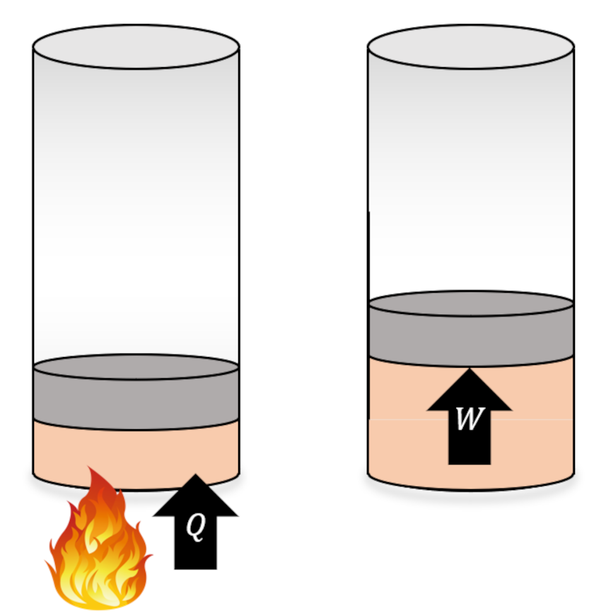
Over the past three posts, we’ve laid the groundwork for the mathematical formulation of entropy. The logic started with two separate but equivalent formulations of the second law: Kelvin’s postulate and Clausius’ postulate. Both postulates summarize some aspect of those processes that never occur even though the first law (conservation of energy) doesn’t forbid them. The Kelvin postulate says that we can never use a cyclic process to convert any energy extracted as heat from a reservoir into work. Likewise, the Clausius postulate says that we can’t use a cyclic process to make energy flow from a colder system to a warmer one without expending some energy in the form of work during the process. The Carnot cycle is integral in proving that these two postulates are different facets of the same second law, which colloquially has often been characterized as saying that there is no such thing as a free lunch.
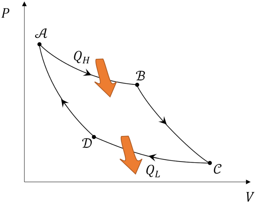
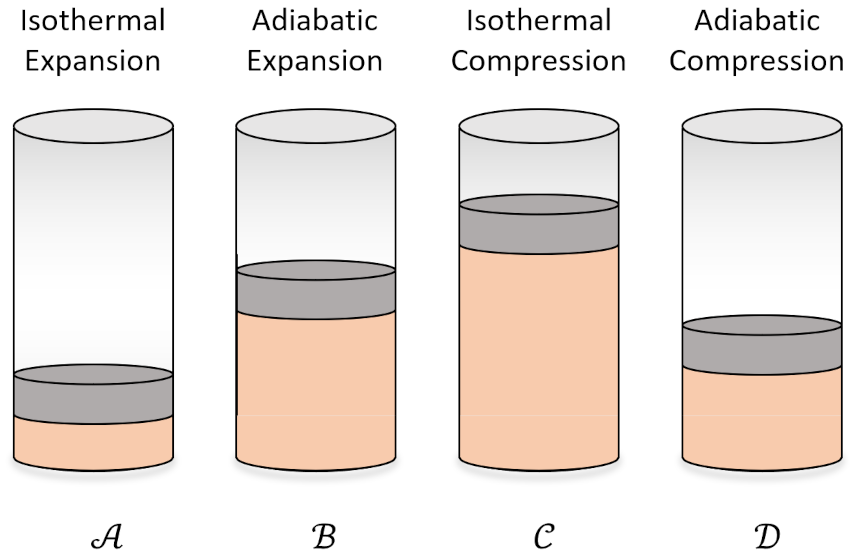
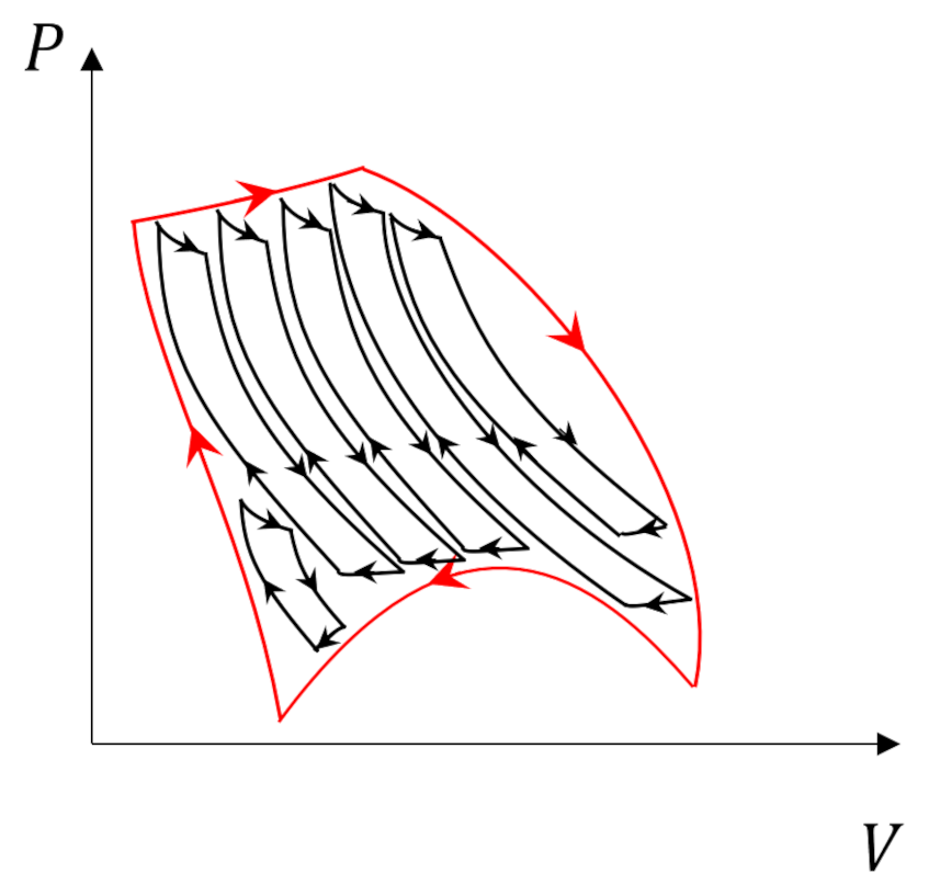
The Carnot cycle has additional responsibilities as a central player in our thermodynamic drama. It’s reversible legs of adiabatic expansion and compression punctuated by isothermal counterparts sets a limit on the efficiency of any engine (Kelvin) or refrigerator (Clausius). So, it shouldn’t be a surprise that it still has additional roles it needs to play. One such role, which was touched on in the post entitled Carnot Cycle, is as the basic ‘atom’ that can used to decompose more complicated cycles.
We are going to use this property to prove two things: 1) the Clausius inequality that further defines the role that entropy plays in descriptions of the second law and 2) that entropy is a state variable.
The arguments presented here closely follow those found in Enrico Fermi’s Thermodynamics supplemented with ideas from Ashley Carter’s Classical and Statistical Thermodynamics.
We start by imaging a cyclic process in which a system interacts with $N$ thermal reservoirs at temperatures $T_1, T_2, \ldots, T_N$. In some of these interactions the system’s temperature $T_S$, which varies throughout the cycle, will be higher than the reservoir temperature and the system will deliver heat in the amount $Q_i$ to the reservoir. In others, $T_S < T_i$ and the system will absorb heat in the amount $Q_i$ from the reservoir. The quantities $Q_i$ will be negative when the energy flows out of the system and positive when energy flows in.
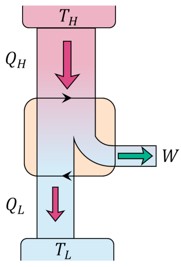
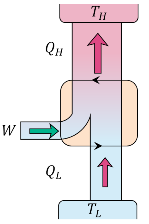
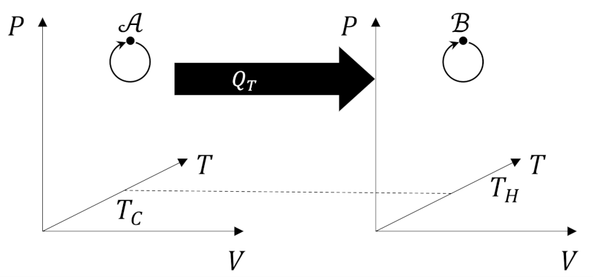
The Carnot decomposition begins by imaging another thermal reservoir, called the base, with temperature $T_0$, which, without loss of generality, is taken to higher than any other temperature in the problem. At each stage of the system cycle, we place a Carnot cycle into contact with the $i^{th}$ reservoir and the base. If the system absorbs heat from the $i^{th}$ reservoir we run the Carnot cycle as an engine extracting work $W_i$ from the energy transfer from the base to the $i^{th}$ reservoir. The following figure shows an example of this type of interaction.
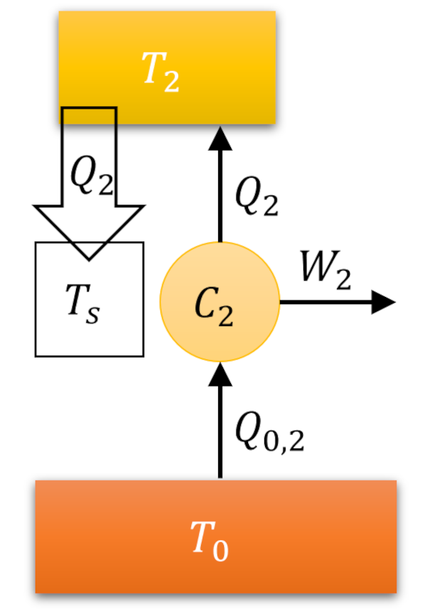
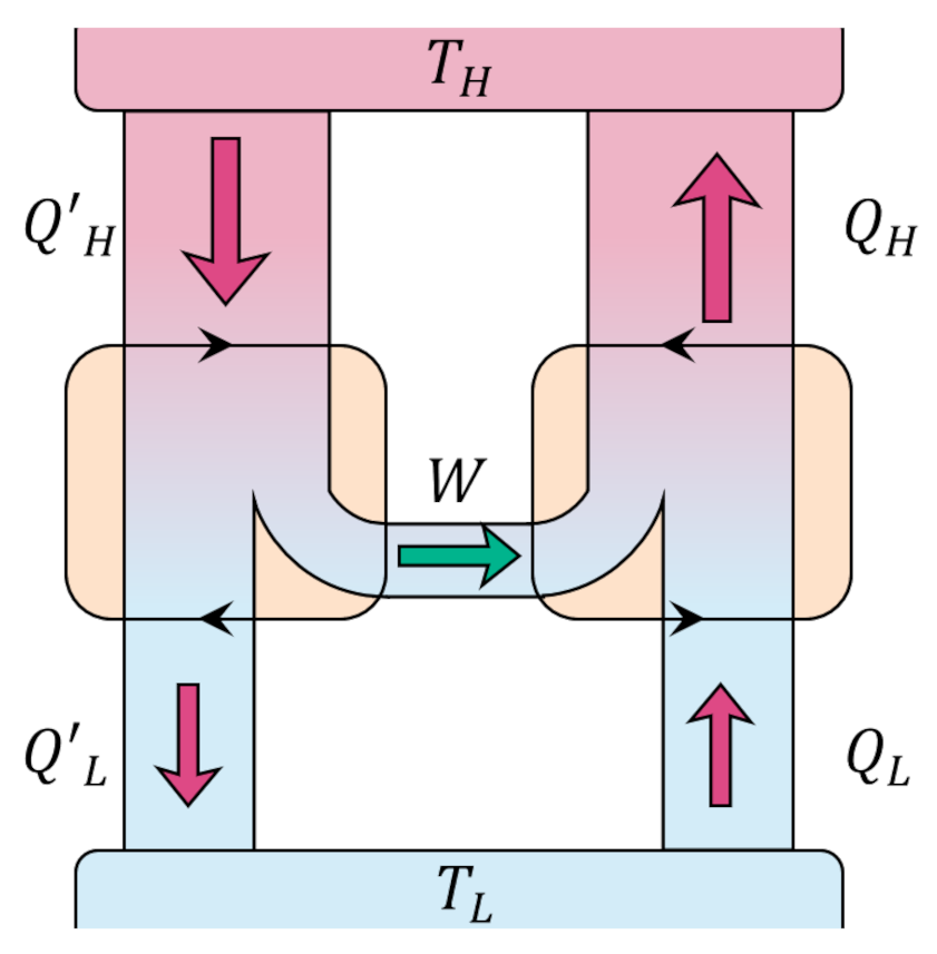
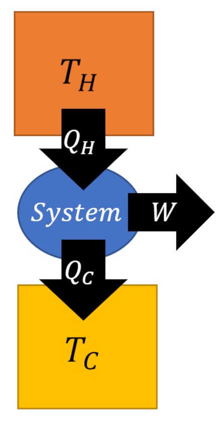
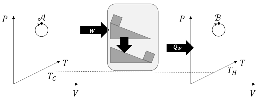
When the system delivers heat to the $i^{th}$ reservoir we run the Carnot cycle as a refrigerator consuming some work $W_i$ to extract the same amount of heat from the reservoir and dump it (and excess heat) into the base.
The following animation shows three turns through what we dub the Fermi Cycle in which our system interacts with 6 reservoirs. Blue-shaded reservoirs have temperatures lower than the system temperature at the time of the interaction while yellow-shaded ones have higher temperatures.
By coupling a Carnot cycle to each stage of the interaction, we can relate the heat absorbed or delivered by the system to the heat exchanged between the base and the various reservoirs by
\[ Q_{0,i} = -\frac{T_0}{T_i} Q_i \; ,\]
which is just a relabeling of a relation
\[ \frac{Q_H}{T_H} = \frac{-Q_L}{T_L} \; ,\]
derived in the previous post.
The total heat transferred from the base is
\[ Q_0 = \sum_{i=1}^N -\frac{T_0}{T_i} Q_i = – T_0 \sum_{i=1}^N \frac{Q_i}{T_i} \; . \]
Despite the overall minus sign, it isn’t immediately clear whether $Q_0$ is positive, negative, or zero since the $Q_i$’s can be of any sign. This ambiguity dissolves when we realize that in a full turn through the Fermi cycle, the original system, the helper Carnot cycles, and the individual reservoirs, which collectively can be taken as a ‘black box’ engine, in and of itself, have returned to its initial state. By the first law, the change in this black box’s internal energy is zero and so the heat exchanged (in or out) has to be equal to the work performed (done by or done to) by the base. By Kelvin’s postulate, it is impossible to extract work from the base so the work has to be zero or negative and so we conclude that $Q_0$ is zero and negative as well, leading us to Clausius’ inequality
\[ \sum_{i} \frac{Q_i}{T_i} \leq 0 \; .\]
Before pushing this expression farther, it is instructive to reflect on the physical content of the previous argument. The fact that the work is negative in a complex irreversible engine reflects the engine’s need for a power source to run and the fact that the heat is also negative (since $Q=W$) reflects that such an engine creates heat that it dumps to the environment as a byproduct. Each automobile engine testifies to this.
Only when the engine is truly reversible can we get equality with zero. This is seen from the fact that if the process is reversible then, upon running the cycle in the opposite direction, all the heat values become negative and so the heat moved from the based in the reversed process is
\[ Q_{0,r} = – T_0 \sum{i} \frac{-Q_i}{T_i} = T_0 \sum_{i} \frac{Q_i}{T_i} = – Q_0 \; .\]
But $Q_{0,r}$ must also obey the Clausius inequality and we conclude $Q_{0,r} = Q_{0} = 0$.
While Clausius’ inequality was derived for a discrete set of reservoirs we can imagine transitioning to a continuum as the number is increased without bound but with each exchange shrinking in size. We ‘loosely’ summarize this as
\[ \oint \frac{{\tilde d} Q}{T} \leq 0 \leftrightarrow \sum_{i} \frac{Q_i}{T_i} \leq 0 \; , \]
where the equality is satisfied for reversible processes. Note that the reasons for the tilde on the $d$ within the integral are due to the fact that the heat is not an exact differential.
The final point to note is define the differential entropy of a system as
\[ dS \equiv \frac{{\tilde d} Q}{T} \; .\]
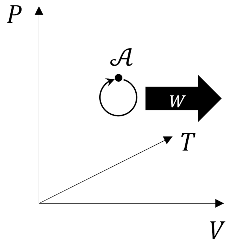
So defined, the entropy is a state variable since any two states, visualized, for example, as points in the $p-V$ can have a value for the change $\Delta S$ unambiguously defined for any reversible process connecting them. The entropy is path independent, otherwise a trip through the cycle would result in zero, and thus, is an exact differential.