
In the spirit of simplicity embraced by the last post, this month’s analysis also deals with motion in one-dimension. As shown in that analysis, the naive application of Newton’s laws to motion of a bead along a curved wire failed except in the simplest of cases – that of motion along a straight line (i.e., essentially down an inclined plane). Instead, Lagrange’s method was used where one of the dynamical degrees of freedom was eliminated by direct substitution of the constraint into the Lagrangian. This post examines another (deceptively) simple problem, the motion of a bob at the end of an ideal pendulum, and compares and contrasts direct substitution of the constraint with the use of Lagrange multipliers. The idea is to examine how Lagrange multipliers work and what information they provide in a problem where one can easily understand all the ‘moving parts’. The content of the post is inspired by the fine write-up on Lagrange multipliers by Ted Jacobson for a course on classical mechanics. I’ve taken Jacobson’s basic discussion on Lagrange multipliers and extended it in several directions; nonetheless, the insights on that particular topic are due to him.
To begin, assume that the pendulum bob can move in the plane subject to the forces of gravity and of an inextensible rod of length $$R$$ to which the bob is attached.
The Lagrangian for arbitrary two-dimensional motion, subjected to gravity along the $$x$$-direction, expressed in plane polar coordinates is
\[ L = \frac{1}{2} m \left( \dot \rho^2 + \rho^2 \dot \phi^2 \right) + m g r \cos \phi \; , \]
where the zero of the potential energy is taken to be the lowest point in the bob’s motion and where the constraint $$\rho = R$$ has not yet been used.
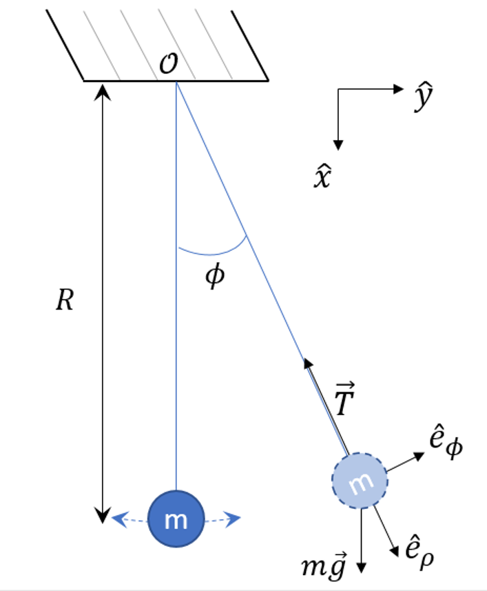
Before digging into the Lagrangian method, it is worth taking a step back to see how this system is described in the Newtonian picture. The forces on the bob at any given point of the motion in the plane lead to a vector equation that is determined by the well-known form of the acceleration in terms of the radial and azimutal unit vectors
\[ \ddot {\vec r} = (\ddot \rho – \rho \dot \phi^2) \hat e_{\rho} + (2 \dot \rho \dot \phi + \rho \ddot \phi) \hat e_{\phi} \; . \]
Applying Newton’s laws to the force vectors shown in the figure gives
\[ m g \cos \phi – T = m (\ddot \rho – \rho \dot \phi^2 ) \; \]
and
\[ -m g \sin \phi = m ( 2 \dot \rho \dot \phi + \rho \ddot \phi )\; .\]
Because the radius is fixed at $$\rho = R$$, the kinematics of the pendulum require $$\dot \rho = 0$$ and $$\ddot \rho = 0$$. The first equation provides a mechanism for calculating $$T$$ as
\[ T = m g \cos \phi + m R \dot \phi^2 \; .\]
The second equation gives the classic equation of motion for the pendulum
\[ R \ddot \phi + g \sin \phi = 0 \; .\]
These simple equations will help in interpretting the Lagrangian analysis.
Directly Impose the Constraint
Since the constraint is holonomic, it can be directly imposed on the Lagrangian, allowing for the radial degree of freedom to be eliminated, yielding
\[ L = \frac{1}{2} m R^2 \dot \phi^2 + m g R \cos \phi \; . \]
The conjugate momentum is
\[ p_{\phi} = m R^2 \dot \phi \; , \]
the generalized force is
\[ Q_{\phi} = – m g R \sin \phi \; , \]
and the resulting equation of motion is
\[ R \ddot \phi + g \sin \phi = 0 \; , \]
exactly the result obtained from Newton’s laws, where computation of $$\hat e_{\rho}$$ and $$\hat e_{\phi}$$ and slogging through a vector set of equations was needed.
It is worth noting how much easier it was to get to these equations than the path through Newton’s laws.
Using Lagrange Multipliers
The alternative way of handling the constraint is by leaving both degrees of freedom (radial and azimuthal) in the Lagrangian, augmenting it with the dynamical constraint. The key is in determining how this augmentation is to be done.
Jacobson argues from analogy with multi-variable calculus. In order to optimize a function $$f(x,y,z)$$ subject to a constraint $$C(x,y,z) = 0$$, one must limit the gradient of the function so that
\[ df = – \lambda d C \; . \]
Since $$C=0$$,
\[ \lambda d C = C d\lambda + \lambda d C = d( \lambda C) \; . \]
This manipulation allows for the combination $$d(f + \lambda C)$$ to now represent an unconstrained optimization problem. In the event there are multiple constraints, each constraint gets a corresponding Lagrange multiplier and is added to the function.
The generalization to variational problems comes by identifying $$f$$ as the action $$S$$. The interesting part is the generalization required to include the constraints. Since the constraint is active at each point of the motion, there are an infinity of constraints, and each one must be included in the action at each time by integration. The resulting unconstrained variational principle is
\[ \int dt (L + \lambda(t) C(t)) \; .\]
The new Lagrangian is
\[ L’ = L + \lambda C = \frac{1}{2} m (\dot \rho^2 + \rho^2 \dot \phi^2) + m g \rho \cos \phi + \lambda (\rho – R) \; . \]
The corresponding radial equation is
\[ m \ddot \rho = m \rho \dot \phi^2 + m g \cos \phi + \lambda \; \]
and the azimuthal equation
\[ m \rho^2 \ddot \phi + 2 m \rho \dot \rho \dot \phi + m g \rho \sin \phi = 0 \; . \]
To these equations must be added the constaint to yield
\[ \lambda = – m \rho \dot \phi^2 – m g \cos \phi \; . \]
and
\[ m R^2 \ddot \phi + m g R \sin \phi = 0 \; . \]
Thus we can identify $$\lambda = T$$, the force of constraint.
This is a general feature of the Lagrange multipliers. They incorporate the constraint into the variation and we are free to ignore it if we want only the dynamics, or we can use $$\lambda$$ to determine if it is explicitly desired.