
In the last two posts, the role of constraints in a mechanical system and the methods for incorporating them have been explored. Among the things that were demonstrated were the facts that the Newton approach was ill-suited to the inclusion of constraints while the Lagrangian method is better equipped, and that within the Lagrangian method there are two approaches for incorporating the constraints: 1) direct elimination in the event the constraints are holonomic, and 2) the use of the Lagrange multipliers. The earlier analysis of the pendulum showed how to analytically use the Lagrange multipliers and demonstrated, in detail, that the multiplier was the force of constraint.
This post returns to the problem of a bead moving down a wire and shows that, whereas the Newtonian approach fails, the Lagrangian approach works nicely. The starting point is the Lagrangian
\[ L = \frac{1}{2} m (\dot x^2 + \dot y^2 ) – m g y + \lambda ( y – f(x) ) \; ,\]
with both $$x$$ and $$y$$ as dynamical degrees of freedom augmented with a Lagrange multiplier that enforces the constraint equation $$y= f(x)$$.
The conjugate momenta are
\[ p_x = \frac{\partial L}{\partial \dot x} = m \dot x \; \]
and
\[ p_y = \frac{\partial L}{\partial \dot y} = m \dot y \; . \]
The corresponding generalized forces are
\[ Q_x = \frac{\partial L}{\partial x} = – \lambda f’ \; ,\]
where $$f’$$ is the derivative of the constraint function $$f(x)$$ with respect to $$x$$, and
\[ Q_y = \frac{\partial L}{\partial \dot y} = – m g + \lambda \; ,\]
The equations of motion are
\[ \ddot x = -\frac{\lambda}{m} f’ \; \]
and
\[ \ddot y = -g + \frac{\lambda}{m} \; .\]
Since the ratio of the Lagrange multiplier to particle mass appears in each equation (i.e., the constraint force per unit mass), it is natural and convenient to define $$\lambda_m = \frac{\lambda}{m}$$ and to work with that quantity going forward.
Since the $$y$$ degree of freedom is related to $$x$$ through the constraint, there is a kinematic relationship that requires
\[ \dot y = \frac{d}{dt} f(x) = \frac{d f}{d x} \frac{dx}{dt} = f’ \dot x \]
and
\[ \ddot y = \frac{d}{dt} \dot y = \frac{d}{dt}( f’ \dot x ) = f” \dot x^2 + f’ \ddot x \; .\]
To determine the Lagrange multiplier, equate the dynamic expression for $$\ddot y$$ with the kinematic one to get
\[ -g + \lambda_m = f” \dot x^2 + f’ \ddot x \; .\]
The next step eliminates the $$x$$ acceleration by substituting-in its equation of motion giving
\[ -g + \lambda_m = f” \dot x^2 – f’^2 \lambda_m \; , \]
which can be easily solved for
\[ \lambda_m = \frac{ f” \dot x^2 + g}{1 + f’^2} \; . \]
This expression of the constraint force per unit mass is similar to the expressions in the earlier analysis but differs in one key way with the inclusion of the velocity-dependent piece proportional to $$\dot x^2$$. This constraint acceleration is now equipped to generate additional force (not just the expected normal force on the surface) as numerical errors move the motion off of the constraint. Of course, this is not a miraculous result and the constraint had been used to link the $$x$$ and $$y$$ equation of motion, but it is cleaner than the earlier method, it provides the constraint force, and, most important, it provides a mechanism for calculating the kinematics in a more convenient way than the solve-for-$$x$$-and-then-deduce method of that earlier post. As a reminder, those state-space equations were
\[ \frac{d}{dt} \left[ \begin{array}{c} x \\ y\\ \dot x \\ \dot y \end{array} \right] = \left[ \begin{array}{c} \dot x \\ \dot y \\ – g \tau f’ \\ – g \tau f’^2 \end{array} \right] \; ,\]
where $$\tau = (1+f’^2)^{-1}$$.
The Lagrange multipliers form of the equations of motion are also easy to code and couple to a standard solver. As in the earlier post, I used the Python and SciPy ecosystem with the primary function being:
def roller_coaster_multipliers(state,t,geometry,g):
    #unpack the state
    x  = state[0]
    y  = state[1]
    vx = state[2]
    vy = state[3]

    #evaluate the geometry
    f,df,df2 = geometry(x)

    #calculate the lagrange multiplier per unit mass
    lam_m = ( df2*vx*vx + g )/(1.0 + df*df)

    return np.array([vx,vy,-lam_m*df,lam_m - g])
where the function geometry can be any curve in the $$x-y$$ plane. For example, for a bead sliding down a parabolic-shaped wire $$y = x^2$$, the corresponding function is
def parabola(x):
    return x**2, 2*x, 2
and the assignment
geometry = parabola
provides this shape to the solver.
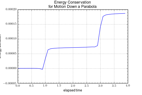
The results for the motion are
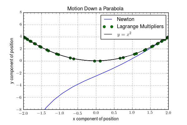
showing excellent agreement with the constraint for over two oscillations and good agreement with energy conservation.
This approach offers a nice alternative to the earlier 1-D approach in that all the dynamical degrees of freedom are present and, as a result, the kinematics are cleaner. In addition, the actual constraint force, taking into account deviations away from the surface, is computed. This is an important feature and one that can’t be obtained otherwise, since we can only compute the normal force at the surface and not away from it on either side.