
This month’s column begins a new chapter in the ongoing study of fluid dynamics. Up to this point, the general equations of fluid motion have been derived from Newton’s laws using the transformation between a fluid-following viewpoint (Lagrangian point-of-view) and a field concept (Eulerian point-of-view). General considerations of mass conservation and the principles of momentum and energy led to a system of non-linear partial differential equations. Ignoring viscosity allowed the equations to simplify to Euler’s equations for an ideal fluid and several specific examples drove home some of the kinematics, dynamics, and methods of solution.
Unfortunately, the situation changes quite dramatically when viscosity is brought back into consideration and the full Navier-Stokes equations (which are themselves something of a simplification) begin to stare back from the page. What is the general mode of attack, and how does one think about the solutions that result? The enormous difficulty of finding solutions becomes even more acute when two facts are driven home. First, it is extremely difficult to find solutions for the simpler set of equations for an ideal fluid, and the solutions shown to date (e.g. the Rankine Vortex), complicated as they may seem, are special cases passed down from one generation to the next precisely because they had a solution. Second, general analytic solutions remain elusive nearly 200 years after Navier first derived these equations in 1822 despite millions of dollars offered to those who could derive such solutions.
To set the stage for an exploration that will consume many columns to come, this installment will present some of the observations and follow many of the arguments gleaned from the article Ludwig Prandtl’s Boundary Layer by John D. Anderson Jr published in the December 2005 issue of Physics Today.
According to Anderson, Ludwig Prandtl
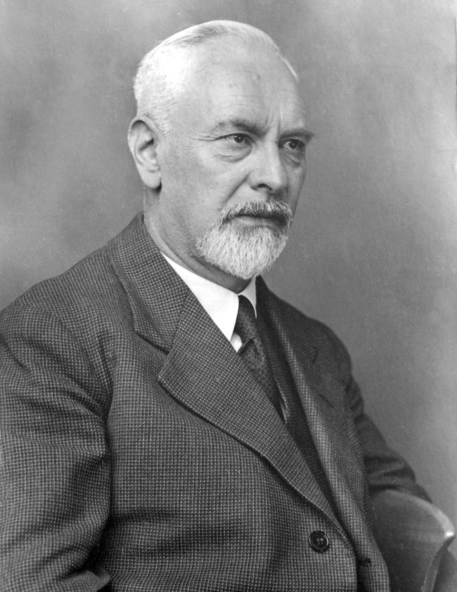
revolutionized fluid dynamics with a very simple to understand and yet highly non-intuitive concept of the boundary layer that exists in a fluid near a rigid surface.
To understand the importance of Prandtl’s result one has to start the story in the latter half of the 18th century, around the time Euler derived the ideal fluid equations bearing his name. The French mathematician Jean le Rond d’Alembert derived a paradox associated with ideal fluid flow. He proved that, for an incompressible fluid with no viscosity (i.e., an ideal fluid), the drag force on an object placed within this flow, moving with constant relative velocity with respect to the fluid, is identically zero, an obviously incorrect result.
Acheson presents a mathematical derivation of d’Alembert’s paradox In Section 4.13 of his book Elementary Fluid Dynamics. This derivation examines the force and momentum balance in the fluid and, using Bernoulli’s streamline theorem, concludes that, for the fluid to be moving at a uniform speed far upstream and far downstream from the body, the drag force on the body must vanish. This result contradicts everyday observations about the motion of solid objects in air or water.
Clearly something was wrong with the theory of ideal fluid, but the specific root of the problem escaped identification for roughly 150 years until Prandtl introduced his boundary layer at a conference in 1904. The modern picture of the boundary layer is best understood in terms of the motion of air over a cambered wing as shown in the figure below (based on Figure 2 of Anderson).
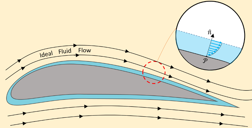
Away from the wing, the ideal fluid model works well in describing the streamlines. However, close to the wing’s surface, viscous effects become dominant in a thin layer whose base attaches to the wing’s surface. This no-slip condition demands that the fluid be at rest at the surface and that the fluid velocity rapidly rise from zero (where the layer attaches to the wing) to the ‘free stream’ velocity of the bulk inviscid flow outside the layer (shown in the inset). In this way, d’Alembert’s paradox is conceptually resolved. The drag force is non-zero, as observed, and the bulk flow is inviscid or ideal (depending on whether one allows the viscosity-free flow to be compressible or not), as observed, but the mathematical conditions by which d’Alembert derived the paradox are not true everywhere – the thin boundary layer makes all the difference.
Prandtl also predicted that, in certain cases, this layer can separate from the surface, which can cause additional drag. To quote Prandtl
Indeed, modern theory classifies the boundary layer behavior as falling into two broad classes. Laminar motion describes the flow when the layer stays fixed to the surface. Turbulent motion describes the flow when the layer separates and produces vortices in wake. Laminar flow produces less drag than turbulent flow but it is unstable and thus harder to produce or control. Turbulence changes the characteristics of the flow far from the surface causing additional drag.
In addition to these two critical physical observations, Anderson points out that the concept of the boundary layer also enabled the first quantitative calculations of aerodynamic drag. The reason for this is that the boundary layer equations exhibit an entirely different type of mathematical behaviors than the equations describing the bulk flow outside. Although both sets of equations are coupled, nonlinear, partial differential equations, the Navier-Stokes equations used to describe the bulk flow external to the layer are elliptic (at least when the flow is subsonic) while the simplification of these equations in the boundary layer are parabolic. This distinction allows the solution methods used to describe the bulk motion to ‘decoupled’ from the methods used to describe the drag and since the methods for solving parabolic equations are much easier to deal with than those for elliptic equations real progress can be made.
What is particularly amazing about Prandtl’s contribution is that the original presentation in 1904 lasted no longer than 10 minutes. I would say that the return on investment resulting from that rather short talk have been nothing short of phenomenal.