
This month’s column deals with viscous flow in a variety of situations. Three main physical effects can drive elementary fluid flow: the pull of gravity coaxing a fluid downhill; a pressure differential, such as in a pipe, causing the fluid to flow from inlet to outlet; or shearing motion, which, in the usual scenario, involves a moving boundary dragging the fluid. We’ll be looking at four examples covering different aspects of these three effects. The first two will illustrate the effect of gravitational body forces and pressure differentials to drive the fluid and will be covered in this column. The next two examples deal with steady and unsteady shear-induced flows and will be featured next month.
But, before we deal with specific examples, we will need to settle on a model of the fluid. Usually, when seeking analytic solutions describing the motion of non-ideal Newtonian fluids (already a simplification compared to the amazingly rich and diverse types of fluids that nature offers), one either chooses to assume the flow is viscous and incompressible or that it is inviscid and compressible. For these examples, we will choose the former.
The starting point will be the incompressible Navier-Stokes equations, of which the flux-conservative form is
\[ \frac{\partial \rho {\vec V}}{\partial t} + \nabla \cdot (\rho {\vec V} {\vec V}) = – \nabla P + \mu \nabla^2 {\vec V} + \frac{1}{3} \mu \nabla \left( \nabla \cdot {\vec V} \right) + \rho {\vec g} \; .\]
Applying the incompressibility assumption ($$\nabla \cdot {\vec V} = 0$$) is easy to do using the Lagrangian form of the equations, but it is more instructive to play with the flux-conservative form. Most of the action takes place on the left-hand side so let’s focus on that by expanding the terms to get
\[ \rho \frac{\partial {\vec V}}{\partial t} + {\vec V} \frac{\partial \rho}{\partial t} + {\vec V} ( {\vec V} \cdot \nabla \rho ) + \rho ({\vec V} \cdot \nabla) {\vec V} + {\vec V} \rho (\nabla \cdot {\vec V}) \; .\]
The last term vanishes under the incompressibility assumption. The second and third terms, combined, are
\[ {\vec V} \left( \frac{\partial \rho}{\partial t} + ( {\vec V} \cdot \nabla ) \rho \right) \; .\]
The quantity in the parentheses vanishes when applying incompressibility to the continuity equation, as follows:
\[ \frac{\partial \rho}{\partial t} + ({\vec V} \cdot \nabla ) \rho + \rho \nabla \cdot {\vec V} = \frac{\partial \rho}{\partial t} + ({\vec V} \cdot \nabla ) \rho = 0 \; ,\]
where the first expression is the full continuity equation and the second is what is left after the incompressibility assumption is applied. The left-hand side is now simply
\[\rho \left( \frac{\partial {\vec V}}{\partial t} + ({\vec V} \cdot \nabla) {\vec V} \right) \;. \]
The third term on the right-hand side vanishes due to the incompressibility assumption. Dividing by the density gives the general form of the Navier-Stokes equations for incompressible fluid flow:
\[ \frac{\partial {\vec V}}{\partial t} + ({\vec V} \cdot \nabla) {\vec V} = – \frac{1}{\rho} \nabla P + \nu \nabla^2 {\vec V} + {\vec g} \; , \]
where $$\nu = \mu/\rho$$ is the kinematic viscosity.
This equation is what we will use in the following examples.
Gravity-driven Flow
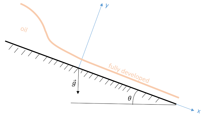
This example derives from the very nice YouTube lecture by Rick Sellens. Here we imagine flow of a fluid, such as oil, down an inclined plane (flow in the $$x$$ direction), as shown in the figure below. The height of the oil is larger at the top of the ramp but it quickly thins as gravity accelerates the oil. Eventually, the viscous force equals the component of the gravitational force parallel to the plane and, thereafter, the height of the oil is constant (the flow is said to be fully developed) and the velocity profile depends only on $$y$$. Once the flow establishes itself, this height profile remains constant in time and the flow is steady, allowing us to set all time derivatives to zero. We will assume that the incline is wide enough in the $$z$$-direction (not pictured) that we can approximate the flow as being two-dimensional. Next, we will confine our description to the fully developed portion of the flow ($$x > 0$$). Finally, we will assume a no-slip boundary condition at the incline plane and, since the flow is open to the air on top and air is not particularly viscous, we will assume the shear stress on the upper surface to be zero.
Applying the steady, fully-developed, and 2-D flow assumptions leads to the continuity equation
\[ \partial_x V_x = 0 \; \]
and the $$x$$- and $$y$$-component Navier-Stokes equations of
\[ 0 = g_x + \nu \frac{\partial^2}{\partial_y^2} V_X \; \]
and
\[ 0 = -\partial_y P + \rho g_y \; ,\]
where $$g_x = g \sin(\theta) $$ and $$g_y = g \cos(\theta)$$, are the components of the gravitational acceleration parallel and perpendicular to the surface of the incline, respectively.
The continuity equation merely confirms what we already assumed, $$V_x = V_x(y)$$. The $$y$$ component of Navier-Stokes says that the pressure at the surface of the incline is higher than at the top due to the weight of the oil above. All the action is in the $$x$$-component equation.
Integrating the equation once yields
\[ \frac{d}{dy} V_x = – \frac{g_x}{\nu} y + C_1 \; . \]
The constant of integration is determined by the shear-stress-free boundary condition at the free surface and gives $$C_1 = g_x h/\nu$$.
Integrating the equation a second time yields
\[ V_x = \frac{g_x}{\nu} \left(h y – \frac{1}{2} y^2 \right) + C_2 \; .\]
The constant of integration is identically zero after the application of the no-slip boundary condition at the incline ($$V_x(y=0)=0$$).
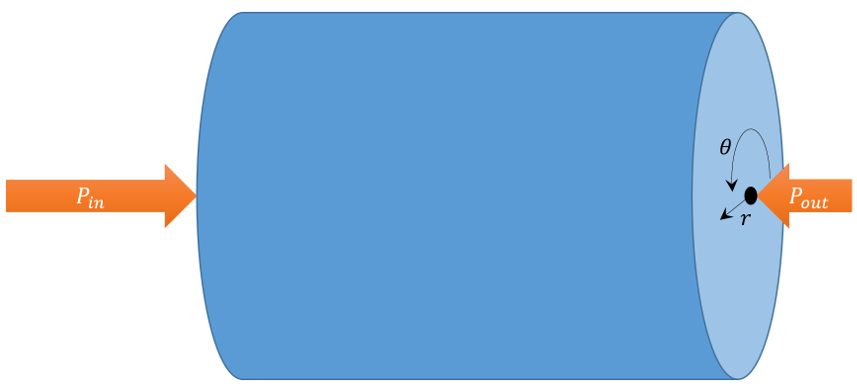
Pressure-driven Flow
This example draws from the Faculty of Kahn video on Poiseuille’s law. In this scenario, we imagine a horizontal pipe with an inlet pressure, $$P_{in}$$, and an outlet pressure, $$P_{out}$$, with $$P_{in} > P_{out}$$ and that the flow has had time to become steady. Cylindrical geometry clearly suggests itself and we expect that the only flow is in the $$z$$-direction ($$V_r = V_{\theta} = 0$$) and its only variation is radial ($$V_z = V_z(r)$$).
As discussed in an earlier post, usually one must take care to differentiate the basis vectors as well as the components when setting up fluid equations in curvilinear coordinates. However, the above assumptions are sufficiently limiting that only the $$z$$-component equation survives in the form
\[ \frac{d P}{d z} = \nu \frac{1}{r} \frac{d}{dr} \left( r \frac{d V_z}{dr} \right) \; . \]
The general solution to this is
\[ V_z(r) = \frac{P_{in} – P_{out}}{4 \mu L} r^2 + C_1 \ln r + C_2 \; .\]
The constants of integration follow from a boundary condition that requires $$V_z(r=0)$$ to be finite and the usual no-slip boundary condition at the walls. The final form is then
\[ V_z(r) = \frac{P_{in} – P_{out}}{4 \mu L}(r^2 – R^2) \; .\]
Integrating this form over the surface area of the pipe gives the famous Poisueille flow rate relationship that says, for a given flow rate, the pressure differential is inversely proportional to the radius to the fourth power. This relationship has profound consequences in the field of medicine.