
Last week, we discussed how a clever interrogation of the Maxwell’s equations to find a variety of relations, including the derivation of Poynting’s theorem. This week, I thought it would be interesting to look a little more at how the Poynting’s theorem works for a set of special cases.
The first case looks at the propagation of the an electromagnetic wave. In this case, common intuition as to the direction of the energy flow will match the mathematics and all looks right with the world. The second case involves a uniform current is put through a resistive wire. This common situation ends up an unusual interpretation of the Poynting flux. The third case, which involves running AC current through a capacitor in a circuit, common intuition about the direction of $$\vec S$$ turns out to be quite wrong and the result is both puzzling and instructive.
On note, before the dissection of the two cases begins. This post is heavily influenced by Chapter 10 in Electromagnetic Theory by Frankl and the discussion in Chapter 27 of the Feynman Lectures on Physics.
Case 1 – Propagation of an Electromagnetic Wave
One of the most celebrated results of Maxwell’s synthesis of the equations that bear his name and which follows from and, in some sense, motivated his inclusion of the displacement term in Ampere’s law is the prediction of electromagnetic waves. From the basic equations, a plane electromagnetic wave of frequency $$\omega$$ propagating in the $$k$$-direction (which can point anywhere) is described by
\[ \vec E(z,t) = \vec E_0 e^{i(\vec k \cdot \vec r – \omega t)} \]
for the electric field and by
\[ \vec B(z,t) = \vec B_0 e^{i(\vec k \cdot \vec r – \omega t)} \]
for the magnetic field.
Note that this form assumes that the wave propagates in free space and, therefore, doesn’t interact with matter. Applying Coulomb’s law ($$div(\vec E) = 0$$) gives
\[ \nabla \cdot \vec E = 0 \Rightarrow \vec E_0 \cdot \vec k = 0 \; .\]
Likewise, the application of the Monopole law leads to $$\vec B_0 \cdot \vec k = 0$$. So the electric and magnetic fields are perpendicular to the direction of propagation and since $$\vec S = \vec E \times \vec B / \mu_0$$ the Poynting flux is parallel to $$\vec k$$ just as common intuition indicates. The energy flow is along the direction of propagation.
Note that a careful computation will show that the magnitude of the energy flow is just what elementary wave mechanics would predict.
Case 2 – Current Through a Resistive Wire
In this case, a long straight wire with conductivity $$g$$ carries a current $$I$$ uniformly distributed across it. The relevant geometry is shown in the figure.
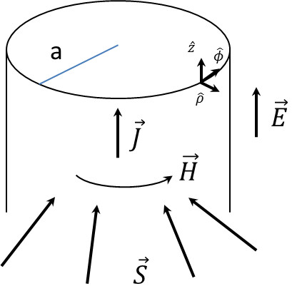
The current density is
\[ \vec J = \frac{I}{\pi a^2} \hat z \; .\]
The electric field needed to drive this current is
\[ \vec E = I R \hat z = I \frac{1}{\pi a^2 g} \hat z \]
and the resulting magnetic field set up by the current (by applying Ampere’s law) is
\[\vec H = \left\{ \begin{array}{c} \frac{I \rho}{2 \pi a^2 } \hat \phi \; \; \text{for} \; \; \rho < a \\ \frac{I}{2 \pi \rho} \hat \phi \; \; \text{for} \; \; \rho >a \end{array} \right. \; , \]
where $$\hat \phi$$ is the unit vector pointing along the azimuthal angle direction and $$\hat \rho$$ points along the radial direction in cylindrical coordinates (i.e. both are confined to the $$x$$-$$y$$ plane in cylindrical coordinates). The Poynting vector evaluates to
\[\vec S = \left\{ \begin{array}{c} -\frac{I^2 R}{2 \pi} \frac{\rho}{a^2} \hat \rho \; \; \text{for} \; \; \rho < a \\ - \frac{I^2 R}{2 \pi} \frac{1}{\rho} \hat \rho \; \; \text{for} \; \; \rho > a \end{array} \right. \; .\]
Note the peculiar nature of the direction of the energy flow. It isn’t along the wire but radially in from the outside.
Now a concern may be raised that there is an error somewhere hidden in the manipulations up to date. To assuage these concerns and build confidence, compute the divergence of the Poynting vector. The result should be related to the energy dissipation happening due to the resistance. The divergence is (recall that, in cylindrical coordinates, $$\nabla \cdot (A_{\rho} \hat \rho) = \frac{1}{\rho} \partial_{\rho} (\rho A_{\rho})$$) :
\[\nabla \cdot \vec S = \left\{ \begin{array}{c} -\frac{I^2 R}{\pi a^2} \; \; \text{for} \; \; \rho < a \\ 0 \; \; \text{for} \; \; \rho > a\end{array} \right. \; . \]
The dissipation within the wire is given by
\[ \vec E \cdot \vec J = \frac{I^2 R}{\pi a^2} \; ,\]
and the Poynting theorem is
\[ \nabla \cdot \vec S + \partial_t u = – \vec E \cdot \vec J \; .\]
Since the situation is static, all partial time derivatives are zero and we should see that $$\nabla \cdot \vec S = – \vec E \cdot \vec J$$, which happily is the result. So, despite what may seem to fly in the face of intuition, the theory holds together.
Case 3 – Run AC Current Through a Capacitor
This case is an intermediate case between the previous two, in which a low-frequency current is driven through a capacitor. This situation is intermediate between the first two – it does not involve static fields but does confine the action to a local circuit element. The relevant geometry is shown in the following figure.
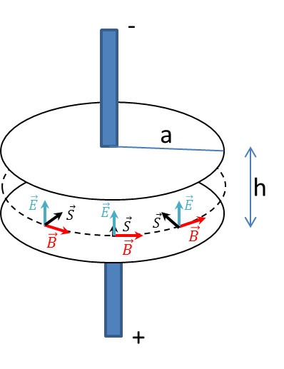
Assuming that the frequency is small enough to ignore the energy in the magnetic field, the total energy contained between the plates is
\[ U_{tot} = u \cdot Vol = (\frac{1}{2} \epsilon_0 E^2)(\pi a^2 h) \]
and it changes as function of time as
\[ \partial_t U_{tot} = \epsilon_0 \pi a^2 h E \partial_t E \; .\]
From an application of Ampere’s law applied to the surfaces of the capacitor, converting the surface integral over $$curl(\vec B)$$ to a line integral along the boundary and using $$\mu_0 \epsilon_0 = 1/c^2$$, yields
\[ 2 \pi a c^2 B = \partial_t E \pi a^2 \; ,\]
which solved for $B$ gives
\[ B = \frac{a}{2 c^2} \partial_t E \; .\]
The direction of $$\vec E$$ is along the axial direction of the capacitor and the direction of $$\vec B$$ is azimuthal. From these facts, it is obvious that the Poynting vector must be pointing radially inward, as shown in the figure.
The magnitude of the Poynting vector is (note the simplification since the electric and magnetic field are perpendicular)
\[ |\vec S| = |\vec E| |\vec B| =\frac{1}{\mu_0} E \frac{a}{2 c^2} \partial_t E = \frac{1}{2} \epsilon_0 a E \partial_t E \; . \]
The total energy flow in is given by the product of the magnitude of the Poynting vector times the total surface area
\[ \Delta U = |\vec S| \cdot Area = (\frac{1}{2} \epsilon_0 a E \partial_t E) (2 \pi a h) = \epsilon_0 \pi a^2 h E \partial_t E \; , \]
which is happily the same result we got above.
So once again, the flow of the energy seems counterintuitive but the results that follow agree with what is expected.