
Wave motion is ubiquitous; from the sound waves we use to hear, to waves on a string instrument, from water waves in the ocean, to light waves from the nearest lamp. The universe presents countless examples of waving phenomena. And yet wave motion is often difficult to understand. This month’s column discusses an interesting aspect of waves that I had not fully appreciated until I was casually reading through Electricity and Magnetism for Mathematicians: A Guided Path from Maxwell’s Equations to Yang-Mills by Thomas A. Garrity.
Bought on a whim, I thought I might get some insight into how mathematicians see electricity and magnetism, specifically, and physics, in general, from the book. Their perspective is generally quite different from that of physicists, since their focus is mostly on rigor and the machinery (how a conclusion is obtained) rather than the particular physical basis for that conclusion. In the past, I have uncovered some useful nuggets on physics from similar texts.
Well, I didn’t have to wait long to uncover one from Garrity. In his chapter 3 on electromagnetic waves, I found a derivation on the nature of the wave equation under Galilean transformations that I hadn’t seen or, perhaps, hadn’t appreciated before.
Physics textbook discussions of the Galilean transformation of the wave equation carry through the transformation of the partial derivative from one frame to the other. In doing so, a mixed second-order term emerges and the derivations I’ve seen stop there with the statement that Galilean transformations ruin the form of the wave equation. But, as Garrity shows, there is an additional step that one can make, and that one step reveals a lot of structure.
To start, consider the wave equation in one dimension
\[ c^2 \frac{\partial^2 f}{\partial x^2} – \frac{\partial^2 f}{\partial t^2} = 0 \; .\]
As is well known, a function of the form $$f(x \pm ct)$$ is a solution to the wave equation. This is most easily seen by defining $$p_{\pm} = x \pm c t$$ and using the chain rule where each of the space or time derivatives is mapped to derivatives with respect to $$p_{\pm}$$.
The first derivatives are
\[ \frac{\partial f}{\partial x} = \frac{d f}{d p_{\pm}}\frac{\partial p_{\pm}}{\partial x} = \frac{d f}{d p_{\pm}} \]
and
\[ \frac{\partial f}{\partial t} = \frac{d f}{d p_{\pm}}\frac{\partial p_{\pm}}{\partial t} = \pm c \frac{d f}{d p_{\pm}} \; .\]
The second derivatives are
\[ \frac{\partial^2 f}{\partial x^2} = \frac{d}{d p_\pm} \left( \frac{d f}{d p_{\pm}} \right)\frac{\partial p_{\pm}}{\partial x} = \frac{d^2 f}{d p_{\pm}^2} \]
and
\[ \frac{\partial^2 f}{\partial t^2} = \frac{d}{d p_{\pm}} \left( \pm c \frac{d f}{d p_{\pm}} \right)\frac{\partial p_{\pm}}{\partial t} = c^2 \frac{d^2 f}{d p_{\pm}^2} \; .\]
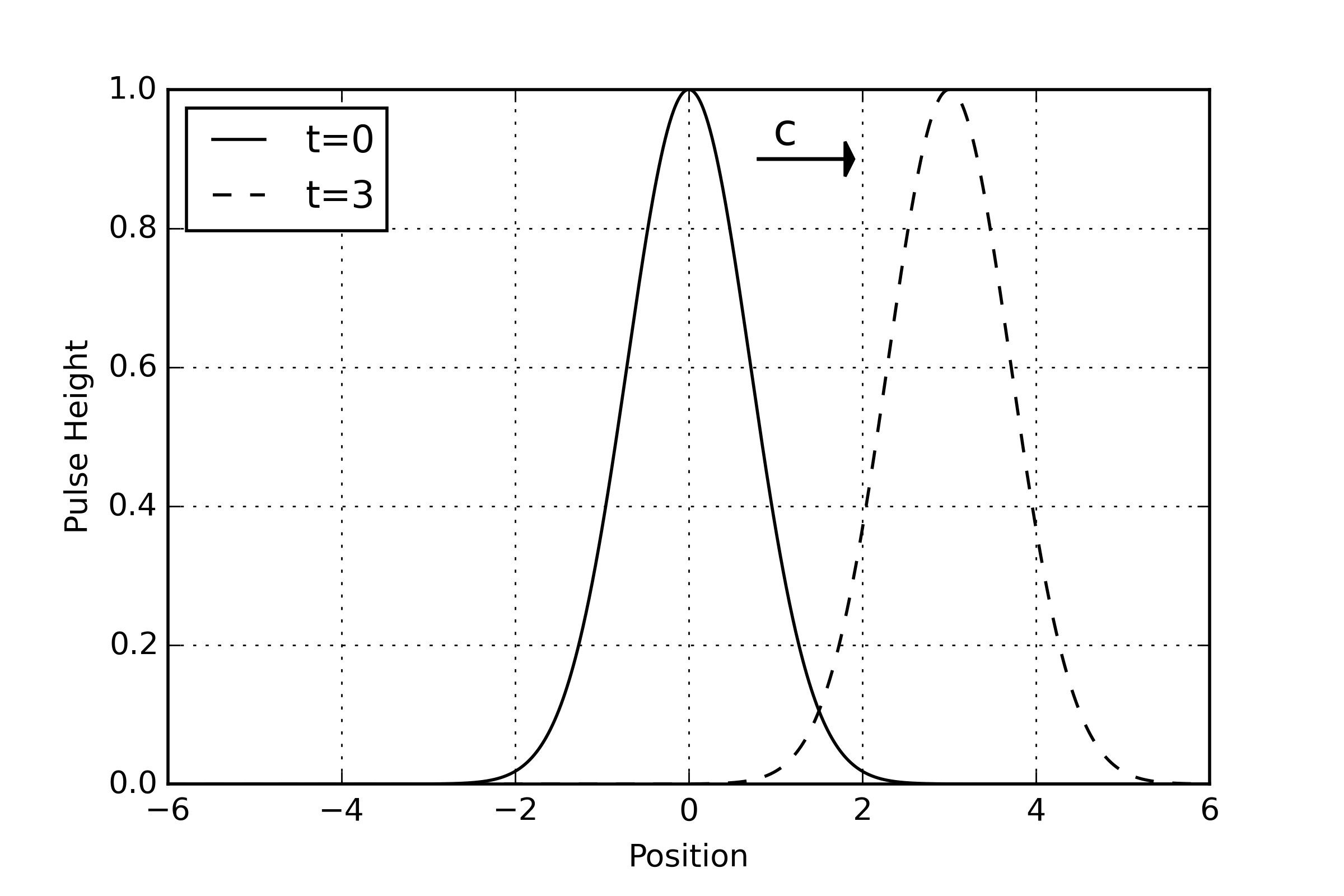
Using this construction, arbitrarily complex waveforms can be constructed without the bother of decomposing them into their Fourier components. For example, the Gaussian pulse
\[ f(x-ct) = e^{-(x-ct)^2} \]
is an exact solution of the wave equation with a pulse height that propagates to the right with a velocity $$c$$.
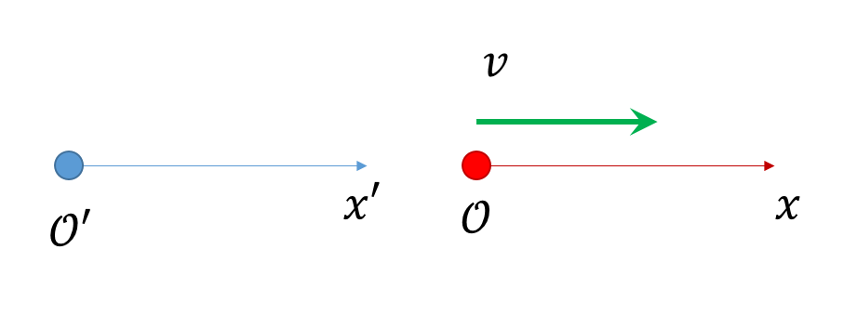
Now suppose that this pulse is propagated along a long string at rest in the frame of an observer $${\mathcal O}$$ and that it persists for a long period of time (i.e. $$c \, t << L$$), so that it can be properly observed. Further, suppose that that string is aboard a moving train that propagates with velocity $$\pm v$$ with respect to an observer $${\mathcal O}'$$ who watches from the ground. The ground-based observer $${\mathcal O}'$$ should be able to conclude that the pulse propagates at speed $$c \mp v$$, without knowing anything about strings, waves, or calculus. The operative question thus becomes whether or not the wave equation supports that conclusion.
To decide, the behavior of the wave equation under a Galilean transformation is required.
The transformation linking observations made by $${\mathcal O}’$$ to those made by $${\mathcal O}$$ are
\[ x’ = v t + x \]
and
\[ t’ = t \; ,\]
with the inverse transformations given by
\[ x = x’ – v t’ \]
and
\[ t = t’ \; .\]
The strategy consists of using the chain rule to express the derivatives in observer $${\mathcal O}$$’s frame to those in the frame of $${\mathcal O}’$$. The first derivatives are:
\[ \frac{\partial f}{\partial x} = \frac{\partial f}{\partial x’}\frac{\partial x’}{\partial x} + \frac{\partial f}{\partial t’}\frac{\partial t’}{\partial x} = \frac{\partial f}{\partial x’} \]
and
\[ \frac{\partial f}{\partial t} = \frac{\partial f}{\partial x’}\frac{\partial x’}{\partial t} + \frac{\partial f}{\partial t’}\frac{\partial t’}{\partial t} = v \frac{\partial f}{\partial x’} + \frac{\partial f}{\partial t’} \; . \]
The second spatial derivative follows immediately as
\[ \frac{\partial^2 f}{\partial x^2} = \frac{ \partial^2 f}{\partial x’^2} \; .\]
The second time derivative is a bit more complicated and is best handled in steps. Substitute in for the first derivative to get
\[ \frac{\partial^2 f}{\partial t^2} = \frac{\partial }{\partial t} \left( v \frac{\partial f}{\partial x’} + \frac{\partial f}{\partial t’} \right) \; .\]
Treating the term in parentheses as a new function $$f$$, the rule used above applies again and a subsequent expansion and collection of terms arrives at
\[ \frac{\partial^2 f}{\partial t^2} = v^2 \frac{\partial^2 f}{\partial x’^2} + 2 v \frac{\partial^2 f}{\partial x’ \partial t’} + \frac{\partial^2 f}{\partial t’^2} \; .\]
Combining the two derivatives gives the wave equation in the frame of $${\mathcal O}’$$ as
\[ (c^2 – v^2) \frac{\partial^2 f}{\partial x’^2} – 2 v \frac{\partial ^2 f} {\partial x’ \partial t’} – \frac{\partial^2 f}{\partial t’^2} = 0 \; . \]
Note the mixed second-order term; this is exactly where most textbooks stop.
But for a right moving pulse, $$f(x-c\,t)$$, the first derivatives are related by
\[ \frac{\partial f}{\partial x} = \frac{d f}{d p_+} \; ,\]
\[ \frac{\partial f}{\partial t} = -c \frac{d f}{d p_+} \; ,\]
and
\[ c \frac{\partial}{\partial x} = -\frac{\partial}{\partial t} \; .\]
Using this relation eliminates that mixed term. First, using the rules derived above, eliminate the partial derivatives in the unprimed frame in favor of those in the primed frame to get
\[ c \frac{\partial}{\partial x’} = – v \frac{\partial}{\partial x’} – \frac{\partial}{\partial t’} \; .\]
Lastly, eliminate the time derivative in the second-order mixed term in favor of the space derivative to yield
\[ (c^2 – v^2) \frac{\partial^2 f}{\partial x’^2} + 2(c+v)v \frac{\partial f^2}{\partial x’^2} – \frac{\partial^2 f}{\partial t’^2} = 0 \; .\]
The two terms multiplying the second-order space derivative can be combined
\[ c^2 – v^2 + 2cv + 2 v^2 = c^2 + 2cv + v^2 = (c+v)^2 \]
and the wave equation becomes
\[ (c+v)^2 \frac{\partial^2 f}{\partial x’^2} – \frac{\partial^2 f}{\partial t’^2} = 0 \; .\]
From basic notions of relative motion, observer $${\mathcal O}’$$ would expect a right-moving wave moving with speed $$c$$ in $${\mathcal O}$$’s frame to move at speed $$c+v$$ and that is exactly what the wave equation asserts.
For a left-moving pulse ($$f = f(x+ct)$$), the signs change a bit:
\[ \frac{\partial f}{\partial x} = \frac{\partial f}{\partial p_-} \; ,\]
\[ \frac{\partial f}{\partial t} = + c \frac{\partial f}{\partial p_-} \; , \]
and
\[ c \frac{\partial}{\partial x} = \frac{\partial}{\partial t} \; .\]
Similar manipulations then lead to the corresponding relation in $${\mathcal O}’$$
\[ \frac{\partial }{\partial t’} = (c-v) \frac{\partial}{\partial x’} \]
and the analogous wave equation
\[ (c-v)^2 \frac{\partial^2 f}{\partial x’^2} – \frac{\partial^2 f}{\partial t’^2} = 0 \; .\]
Again, basic notions of relative motion demand that observer $${\mathcal O}’$$ sees a left-moving wave with speed $$c$$ in $${\mathcal O}$$’s frame to move at speed $$c-v$$ and that is exactly what the wave equation gives.