
This post, building on the work of the previous two posts, investigates the six cases possible in which $$E=h$$ or $$E\neq h$$ and in which either one, the other, neither, or both are conserved. The examples are generally taken from simple mechanical systems in an attempt to illustrate the underlying physics without bringing in an unwieldy set of mathematics.
As a reminder, the energy $$E$$ is always defined as the sum of kinetic and potential energies and the function $$h$$ reflects not only the underlying physics (i.e., $$E$$) but also the generalized coordinate system in which it is described. The power of the generalized coordinates will allow us, in certain circumstances, to find conserved energy-like quantities that are not the energy proper. This is the power and complexity of generalized coordinates and it is this feature that makes it fun.
Case 1 – $$E \neq h$$, both conserved: Free Particle with Co-moving Transformation
Consider the free particle. The Lagrangian for the system is given by
\[ L = \frac{1}{2} m {\dot x}^2 \; .\]
The conjugate momentum and the generalized force are
\[ p_x = m {\dot x} \]
and
\[ \Phi_x = \frac{\partial L}{\partial x} = 0 \; , \]
respectively. The equation of motion is the familar
\[ m \ddot x = 0 \; ,\]
leading to the usual solution
\[ x(t) = x_0 + v_0 t \; .\]
The conserved quantity $$h_x$$ is the energy, which is entirely kinetic, given by:
\[ h_x = \dot x p_x – L = \frac{1}{2} m v_0^2 = E\; .\]
Now suppose that we define the generalized coordinate $$q$$ through the transformation $$x = q + v_0 t$$ and $$\dot x = \dot q + v_0$$. The corresponding Lagrangian is
\[ L = \frac{1}{2} m \left(\dot q + v_0 \right)^2 \]
with the corresponding equation of motion
\[ m \ddot q = 0 \; . \]
The conserved quantity $$h_q$$ is given by
\[ h_q = \dot q p_q – L = m \dot q (\dot q + v_0) – \frac{1}{2} m (\dot q + v_0)^2 = \frac{1}{2} m \dot q^2 – \frac{1}{2} m v_0^2 \; .\]
From the transformation equation, $$q = v_0$$ and so $$h_q = 0$$. The physical interpretation is that, by transforming (via a Galilean transformation) into a frame co-moving with the free particle, the conserved quantity is identically zero, a value different from the energy in the original frame.
Case 2 – $$E \neq h$$, $$E$$ conserved: Free Particle with Accelerating Transformation
Building off of the last case, again look at the free particle and consider the transformation into an accelerating frame given by
\[ x = q + \frac{1}{2} a t^2 \; ,\]
with
\[ \dot x = \dot q + a t \; .\]
The transformed Lagrangian is
\[ L = \frac{1}{2} m \left( \dot q + a t \right) ^2 \; . \]
The corresponding $$h_q$$ is
\[ h_q = m \dot q (\dot q + a t) – \frac{1}{2} m \left(\dot q + a t \right)^2 = \frac{1}{2} m \dot q^2 – \frac{1}{2} m a^2 t^2 \; , \]
which, since it is time varying, is not conserved.
Case 3 – $$E = h$$, both conserved: Planar SHO
An example where the value of the energy $$E$$ and the function $$h_q$$ can take on dramatically different forms and yet yield the same value is supplied by the planar simple harmonic oscillator. In this case, a mass is found in cyclindrically symmetric harmonic potential $$V = 1/2 \, k(x^2 + y^2)$$.
The corresponding Lagrangian is given by
\[ L = \frac{1}{2} m \left( {\dot x}^2 + {\dot y}^2 \right) – \frac{1}{2} k \left( x^2 + y^2 \right) \; , \]
with the equation of motion being
\[ m \ddot {\vec r} = -k \vec r \; .\]
This equation has well known analytical solutions, but for a change of pace, I implemented numerical solutions of these equations with a Jupyter notebook. The state-space equation took the form of
\[ \frac{d}{dt} \left[ \begin{array}{c} x \\ \dot x \\ y \\ \dot y \end{array} \right] = \left[ \begin{array}{c} \dot x \\ – k/m \; , x \\ \dot y \\ -k/m \; , y \end{array} \right] \; . \]
Under the point transformation to plane polar coordinates
\[ x = r \cos ( \omega_0 t) \]
and
\[ y = r \sin ( \omega_0 t) \; ,\]
(where $$\omega_0 = \sqrt{k/m}$$), the Lagrangian becomes
\[ L = \frac{1}{2} m \left( {\dot r}^2 + r^2 {\dot \theta}^2 \right) – \frac{1}{2} k r^2 \; .\]
The resulting Euler-Lagrange equations are
\[ m \ddot r + k r = 0 \]
and
\[ \frac{d}{dt} \left( m r^2 \dot \theta \right) = 0 \; , \]
which are interpretted as the equation of motion of a one-dimensional radial oscillator and the conservation of the angular momentum in the $$x-y$$ plane. The corresponding numerical form is
\[ \frac{d}{dt} \left[ \begin{array}{c} r \\ \dot r \\ \theta \\ \dot \theta \end{array} \right] = \left[ \begin{array}{c} \dot r \\ – k/m \, r + r \dot \theta^2 \\ \dot \theta \\ -2 \dot r \dot \theta /r \end{array} \right] \; . \]
The initial conditions for the simulation were
\[ {\bar S}_0 = \left[ \begin{array}{c} R \\ 0 \\ 0\\ R \omega_0 \end{array} \right] \]
and
\[ {\bar S}_0 = \left[ \begin{array}{c} R \\ 0 \\ 0\\ \omega_0 \end{array} \right] \; ,\]
for Cartesian and polar forms, respectively.
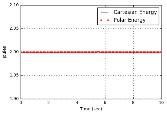
After the trajectories had been computed, the ephemerides were fed into functions that computed the Cartesian energy
\[ E = \frac{1}{2} m \left( {\dot x}^2 + {\dot y}^2 \right) \]
and
\[ E = \frac{1}{2} m \left( {\dot r}^2 + r^2 {\dot \theta}^2 \right) \; ,\]
as appropriate. As expected, the values for the energy, arrived at in two independent ways, are identical
Case 4 – $$E \neq h$$, $$h$$ conserved: Constrained Planar SHO
In constrast to the Case 3, the constrained planar simple harmonic oscillator executes its motion subject to the constraint
\[ {\dot \theta} = \omega \; ,\]
where $$\omega$$ is the driving frequency. The mechanical analog would be something like the following picture
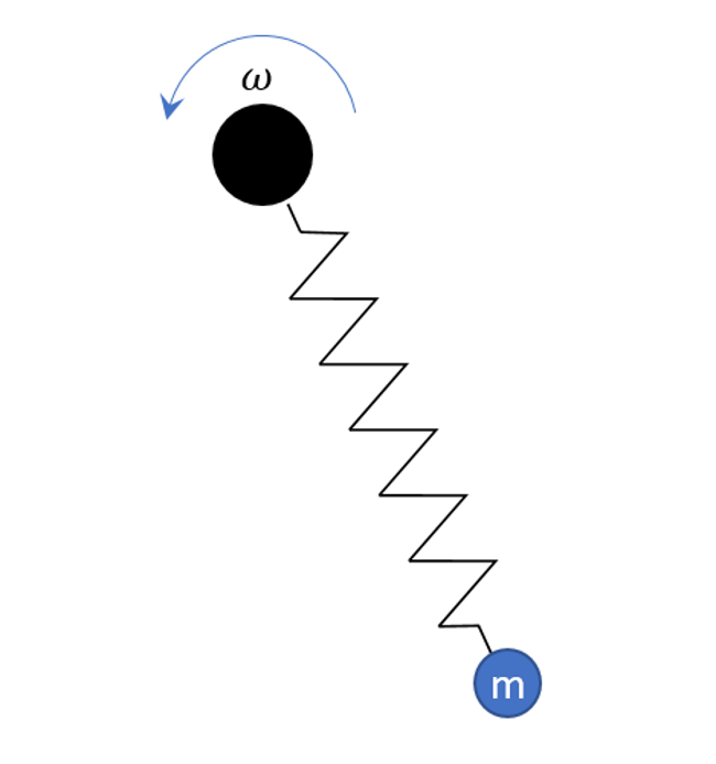
where a mass on a spring is forced by a motor that keeps the oscillator rotating at a constant angular rate.
The Lagrangian in this case is given by
\[ L = \frac{1}{2} m \left( {\dot r}^2 + r^2 \omega^2 \right) – \frac{1}{2} m k (r-\ell_0)^2 \; . \]
Note that there is no easy way to express the Lagrangian in Cartesian coordinates – another example of the power of generalized coordinates.
The energy of the system is
\[ E = T + U = \frac{1}{2} m \left( {\dot r}^2 + r^2 \omega^2 \right) + \frac{1}{2} m k (r-\ell_0)^2 \; ,\]
but
\[ h_r = \frac{1}{2} m \left( {\dot r}^2 – r^2 \omega^2 \right) + \frac{1}{2} m k (r-\ell_0)^2 \; . \]
The minus sign makes all the difference here. Since there is a motor in the problem, the expectation is that the energy should not be conserved, even though the structure of Lagrangian mechanics guarentees the conservation of $$h$$ (since it is not time-dependent).
While there are analytic solutions to these equations, I again opted for a numerical simulation. The equation of motion is
\[ {\ddot r} = (\omega^2 – \omega_0^2)r + k \ell_0 \; , \]
where $$\omega_0^2 = k/m$$.
The resulting dynamics show the radial motion oscillating sinusoidally

about an equilibrium value determined by
\[ r = \frac{k \ell_0}{\omega_0^2 – \omega^2} \; . \]
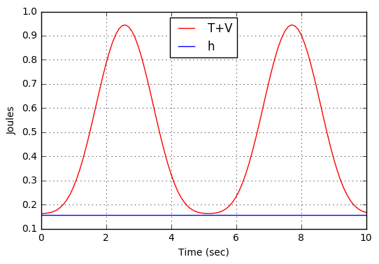
The graph of the energy and $$h_r$$ shows clearly that the energy is not conserved, even though $$h_r$$, as expected, is
Case 5 – $$E \neq h$$, neither conserved: Damped SHO
The final example is the damped simple harmonic oscillator. The Lagragian is given by
\[ L = e^{\gamma t/m} \left[\frac{1}{2} m {\dot x}^2 – \frac{1}{2} k x^2 \right] \; , \]
which results in the equation of motion
\[ m {\ddot x} + \gamma {\dot x} + k x = 0 \; .\]
The energy,
\[ E = \frac{1}{2} {\dot x}^2 + \frac{1}{2} k x^2 \; ,\]
is clearly not conserved and the $$h$$ function,
\[ h = {\dot x} \frac{\partial L}{\partial \dot x} – L = e^{t \gamma/m} E \; ,\]
is also not conserved since it depends on time.
Case 6 – $$E = h$$, neither conserved
This last case is something of a contrivance. As may have been guessed, by the above examples, finding a case where $$E=h$$ and yet both are not conserved is not particularly easy to do. Rotating drivers that leave a dynamical condition like $$\dot \theta = constant \equiv \omega$$ lead to a conserved $$h$$ since the transformation to a rotating frame leaves the system in a co-moving configuration, despite the time varying nature of the transformation. Equally frustrating is trying to incorporate dissipation into the problem. Dissipation generally leads to a different form for $$h$$ compared with $$E$$ as Case 5 demonstrates.
The one example that does work, is by defining the potential energy as
\[ V = x F(t) \]
and the Lagrangian as
\[ L = \frac{1}{2} m {\dot x}^2 – x F(t) \]
resulting in the equation of motion
\[ m {\ddot x} = F(t) \; .\]
Both the energy and $$h$$ are given by
\[ \frac{1}{2} m {\dot x}^2 + x F(t) \; , \]
which is clearly not conserved.