
This month’s posting and the next one are meant to serve as both a final act in the simple kinetic theory that has been the focus in recent columns and to provide a prelude for the more in depth Boltzmann distribution theory that follows. Over the past 8 posts, we’ve explored how simple interactions between constituents of a gas lead to the notion of pressure, help explain the Maxwell-Boltzmann distribution of speeds in the gas at a given temperature, and help us connect measurable, macroscopic features of a material, such a viscosity, to the underlying movement of atoms and molecules. In these final two posts, we’ll look at hard sphere scattering as the specific particle-to-particle interaction and we’ll explore how this simple model directly gives rise to the Maxwell-Boltzmann distribution.
This post will present the mechanical aspects of gas of hard spheres confined to a box and how they are reflected off the walls when they hit (leading to pressure) and how they bounce off of each other when they collide. The subsequent post talks about the aspects of making a kinetic theory simulation and presents the results. The discussion presented here is heavily influenced by and expands and tweaks the very fine simulation by Bruce Sherwood in what was originally known as Visual Python and is now part of Glowscript.org.
There are three basic ingredients in the hard-sphere gas simulation that will be dealt with in turn: 1) the propagation of a sphere between bounces, 2) the bounce off a wall, and 3) the bounce off each other.
Free propagation of each hard sphere between wall and particle interactions is done via simple rectilinear propagation. Assuming that the initial position and velocity of the sphere is ${\vec r}_0$ and ${\vec v}$, then its subsequent location is
\[ {\vec r}(t) = {\vec r}_0 + {\vec v} \cdot (t-t_0) \; . \]
The velocity remains unchanged until collision with a wall or another hard sphere.
When the atoms reach a wall, they bounce elastically with their normal component of velocity being negated. For example, in the example pictured here,
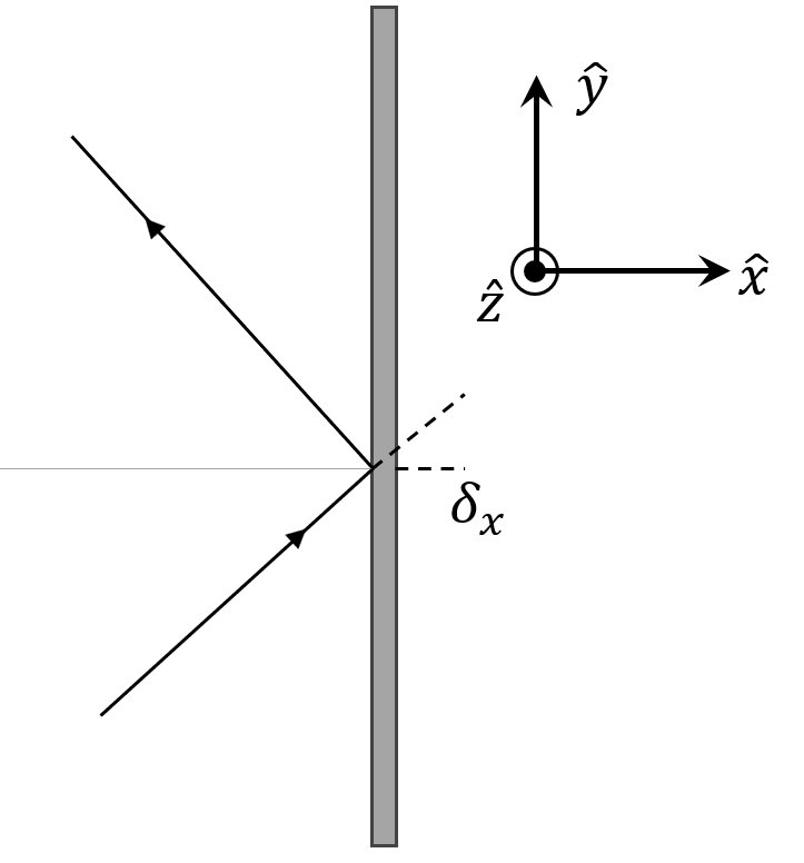
we see a particle approaching a wall in the $y-z$ plane. After the bounce, the $x$-component of the velocity has changed but the transverse components in $y$ and $z$ have not:
\[ {\vec v} = v_x {\hat x} + v_y {\hat y} + v_z {\hat z} \; \rightarrow \; {\vec v} = \, – v_x {\hat x} + v_y {\hat y} + v_z {\hat z} \; .\]
Since time in the simulation elapses in discrete steps, collision with the wall is checked for after each time step. If a component of the particle’s position puts it beyond the confining box (i.e., it passed through a wall at $x = L$ so that its current $x$-component of position is $x = L + \delta_x$ ) then that component of the velocity is negated as above and the distance it had traveled beyond the wall is increment to the appropriate component in the opposite direction (i.e., $x = L – \delta_x$).
The collision between hard spheres is the most complicated part of this simulation. Like the case with the wall, it will often be the case that at the end of a time step, two particles have their hard body radii $R_1$ and $R_2$ overlapping.
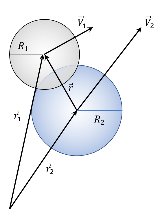
Once this overlapping end condition is detected, the next step is to determine the time $\delta t$ to back up such that the spheres are just touching. The algorithm to determine the time step is most easily understood in a frame in which one of the particles, say $m_2$ in blue, is at the center of the coordinate system and the relative velocity vector ${\vec v} = {\vec v}_1 – {\vec v}_2$ is along the horizontal. Letting ${\vec r} = {\vec r}_1 – {\vec r}_2$ be the relative position of $m_1$ relative to $m_2$ then the unknown quantity is the vector ${\vec d}$ between the current relative position and the relative position ${\vec r}^{\, *}$ when the two spheres are just touching.
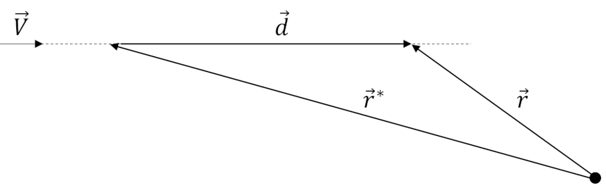
Since ${\vec r}^* + {\vec d} = {\vec r}$ and we know that the length of ${\vec r}^*$ is $R_1 + R_2 = 2 R$ (i.e., $R$ is the average radius) then a quadratic formula can be developed from
\[ |{\vec r}^{\, *}|^2 = |{\vec r} – {\vec d}|^2 \; . \]
After some straightforward algebra, we arrive at
\[ d^2 – 2 r \cos (\theta) d + (r^2 – 4R^2) = 0 \; , \]
where $d = |{\vec d}|$, $r = |{\vec r}|$ and $\cos (\theta) = {\hat r} \cdot {\hat V}$, since the relative velocity ${\vec V}$ is parallel to ${\vec d}$.
Solving for $d$ yields
\[ d = r \cos (\theta) – \sqrt{ 4R^2 + r^2 ( \cos(\theta)^2 – 1 ) } \; , \]
where we picked the negative radical because it guarantees $\delta t$ to be negative signifying that the contact time is in the past as we know it must be.
The final ingredient is to determine how the velocities of the two particles should alter due to their collision. The direction is straightforward as the component of each particle normal to the tangent plane containing their contact must change sign but the magnitude requires a bit more care.
The analysis begins first by calculating the center-of-mass
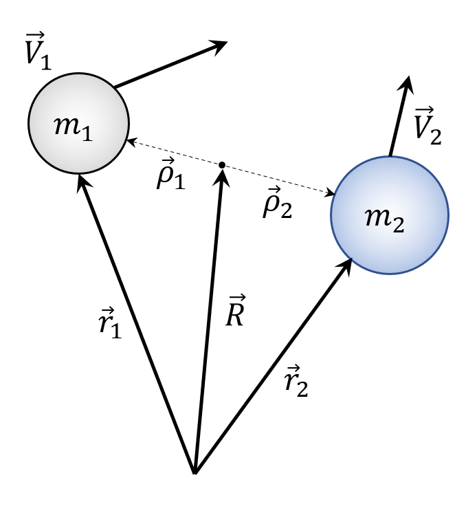
via the usual formula
\[ m_1 {\vec r}_1 + m_2 {\vec r}_2 = M {\vec R} \; . \]
Taking a time derivative of this definition
\[ {\vec p}_1 + {\vec p}_2 = {\vec P}_{tot} = m_1 {\vec v}_1 + m_2 {\vec v}_2 = M {\vec U} \; \]
leads to a useful relationship between the center-of-mass kinematics, defined in terms of the total mass $M$ and the velocity of the center-of-mass ${\vec U}$
\[ {\vec U} = \frac{ {\vec P}_{tot} }{M} \; .\]
The next step is finding the positions, ${\vec \rho}_i$, of both masses relative to the center-of-mass using ${\vec R} + {\vec \rho}_i = {\vec r}_i $ to yield
\[ {\vec \rho}_i = {\vec r}_i – {\vec R} \; . \]
Multiplying by $m_i$, taking the time derivative, and defining the momentum of each mass relative to the center-of-mass as ${\vec \pi}_i = m_i \frac{d}{dt} {\vec \rho}_i$ gives the expression
\[ {\vec \pi}_i = {\vec p}_i – m_i {\vec U} = {\vec p}_i – m_i \frac{{\vec P}_{tot}}{M} \; , \]
where the last equality follows from the earlier relationship between the total momentum and the velocity of the center-of-mass.
The physical interpretation of the ${\vec \pi}_i$ is most clearly revealed by summing them
\[ {\vec \pi}_1 + {\vec \pi}_2 = {\vec p}_1 – m_1 \frac{{\vec P}_{tot}}{M} + {\vec p}_2 – m_2 \frac{{\vec P}_{tot}}{M} \\ = ({\vec p}_1 + {\vec p}_2) – (m_1 + m_2) \frac{{\vec P}_{tot}}{M} = 0 \; .\]
This relation and the one before supply the physical interpretation for the ${\vec \pi}$’s: they are the momenta of each particle in a coordinate frame comoving with the center of mass (i.e., relative to the center-of-mass). The Galilean transform that affects this result is said to have transformed the momenta (or velocity) into the center-of-momentum frame.
The application of the on-contact bounce is trivial in this frame. The total change in momentum is done only in the direction parallel to the line joining the two masses (i.e., normal to the tangent plane containing the contact)
\[ \Delta {\vec p} = ({\vec \pi}_i \cdot {\hat \rho}_i ) {\hat \rho}_i \; \]
and must be equal and opposite for each particle.
Each of the ${\vec \pi}_i$ changes to its after bounce value ${\vec \pi}’_i$ according to
\[ {\vec \pi}’_i = {\vec \pi}_i – 2 \Delta {\vec p} \; .\]
The change in velocity is then found by first reversing the transformation to get ${\vec p}’_i$ via
\[ {\vec p}’_i = {\vec \pi}’_i + m_i \frac{{\vec P}_{tot}}{M} \; , \]
from which immediately follows
\[ {\vec v}’_i = {\vec p}’_i / m_i \; . \]
Next month’s column covers the details of how these theoretical results are translated into a simulation and explores the results.