
Most students find the study of the motion of a rigid body a difficult undertaking. There are many reasons for this and it is hard to rank which one is the greatest stumbling block. Regardless of its rank, fleshing out the relationship between the angular velocity in the body-frame and the angular in the inertial frame is certainly near the top.
First off, the very concept of angular velocity being represented by a vector is foreign concept and difficult to reconcile with the idea that finite rotations are represented by matrices that do not commute. Second, we usually want to express the angular velocity in terms of time derivatives of certain Euler angles and each of these is most naturally expressed in a frame different from all the others.
This short column is intended to give a step-by-step calculation that addresses some of the difficulties encountered in this second point. While the results are not new, the presentation is fairly novel in the pedagogy, which is clean and straightforward.
For sake of concreteness, this presentation will focus on the traditional Euler 3-1-3 sequence used in celestial mechanics to orient the plane of an orbit. This selection has two advantages: it is commonly found in textbooks (e.g. Goldstein) and it involves only two transformation primitives. Its one drawback is that modern attitude control typically uses a different sequence. This latter point may be address in a companion entry at a future date.
We will use the transformation primitives
\[ {\mathcal T}_x(\alpha) = \left[ \begin{array}{ccc} 1 & 0 & 0 \\ 0 & \cos \alpha & \sin \alpha \\ 0 & -\sin \alpha & \cos \alpha \end{array}\right] \; \]
and
\[ {\mathcal T}_z(\alpha) = \left[ \begin{array}{ccc} \cos \alpha & \sin \alpha & 0 \\ -\sin \alpha & \cos \alpha & 0 \\ 0 & 0 & 1 \end{array}\right] \; . \]
The classical Euler 3-1-3 sequence gives a transformation matrix from inertial to body frame expressed as
\[ {\mathcal A} = {\mathcal T}_z(\psi) {\mathcal T}_x(\theta) {\mathcal T}_z(\phi) \; . \]
Before finding the angular velocity in the body frame, an explicit form of the attitude, $${\mathcal A}$$, is needed as it serves two purposes. It is the operator that maps body rates in the inertial frame to the body frame. It is also the device by which we get the intermediate frame orientations during the transformation. These intermediate frames provide the most straightforward route for expressing the Euler angle rates as inertial angular velocity vectors.
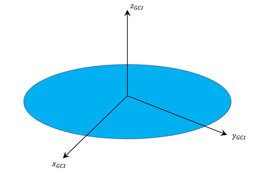
Start with a a known inertial frame here denoted as $$\left\{\hat x_{GCI}, \hat y_{GCI}, \hat z_{GCI} \right\}$$
and begin by applying the operator $${\mathcal T}_z(\phi)$$ corresponding to a tranformation into a frame rotated by an angle $$\phi$$ about $$\hat z_{GCI}$$.
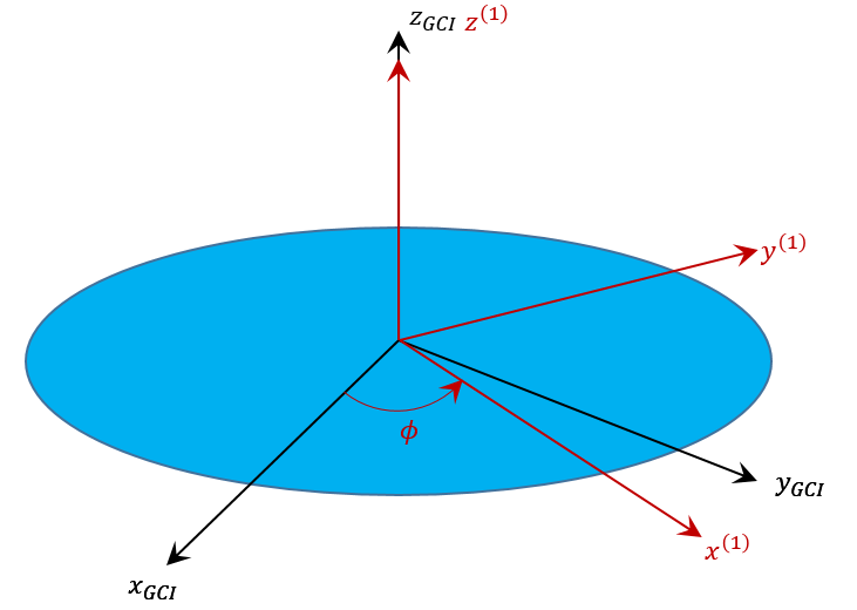
The intermediate transformation matrix
\[ {\mathcal A}^{(1)} = \left[ \begin{array}{ccc} \cos \phi & \sin \phi & 0 \\ -\sin \phi & \cos \phi & 0 \\ 0 & 0 & 1 \end{array}\right] \; \]
allows us to read off the basis vectors in the intermediate frame from the rows of $${\mathcal A}^{(1)}$$:
\[ \hat x^{(1)} = \left[ \begin{array}{c} \cos \phi \\ \sin \phi \\ 0 \end{array} \right]_{GCI} \; ,\]
\[ \hat y^{(1)} = \left[ \begin{array}{c} -\sin \phi \\ \cos \phi \\ 0 \end{array} \right]_{GCI} \; ,\]
and
\[ \hat z^{(1)} = \left[ \begin{array}{c} 0 \\ 0 \\ 1 \end{array} \right]_{GCI} \; .\]
The subscript $$GCI$$ reminds us that these vectors are expressed in the inertial frame even though they point along the axes of the intermediate frame.
Next apply the operator $${\mathcal T}_x(\theta)$$ corresponding to a tranformation into a frame rotated by an angle $$\theta$$ about $$\hat x ^{(1)}$$.
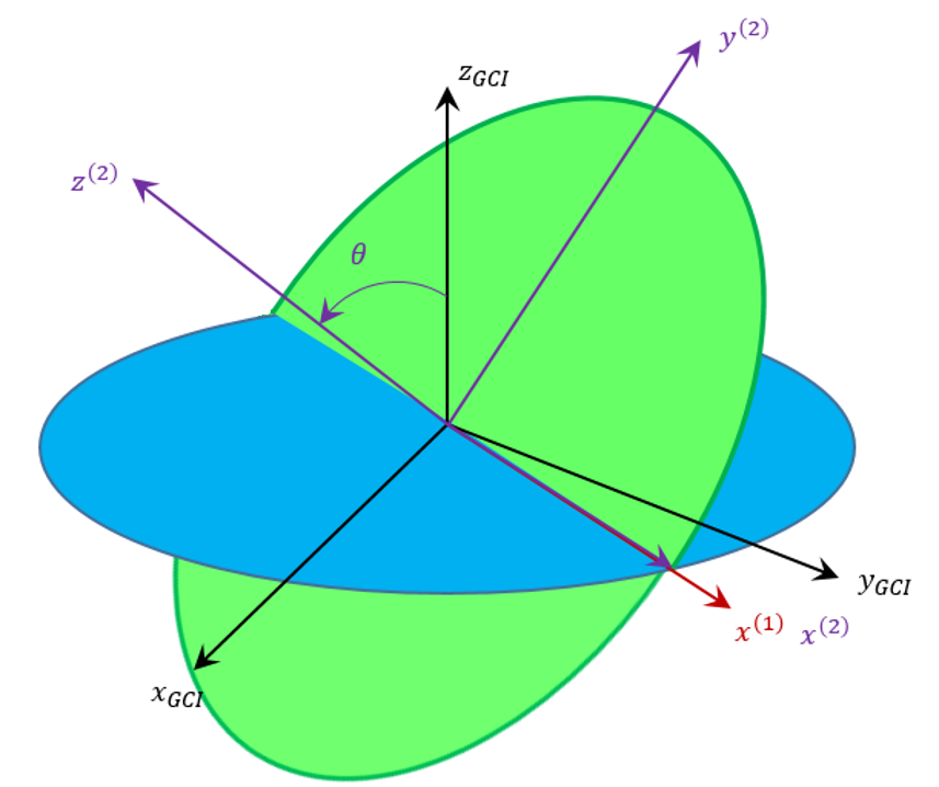
The corresponding intermediate transformation matrix
\[ {\mathcal A}^{(2)} = \left[ \begin{array}{ccc} \cos \phi & \sin \phi & 0 \\ – \sin \phi \cos \theta & \cos \phi \cos \theta & \sin \theta \\ \sin \phi \sin \theta & -\cos \phi \sin \theta & \cos \theta \end{array}\right] \; \]
and the basis vectors in this frame are
\[ \hat x^{(2)} = \left[ \begin{array}{c} \cos \phi \\ \sin \phi \\ 0 \end{array} \right]_{GCI} \; ,\]
\[ \hat y^{(2)} = \left[ \begin{array}{c} -\sin \phi \cos \theta \\ \cos \phi \cos \theta \\ \sin \theta \end{array} \right]_{GCI} \; ,\]
and
\[ \hat z^{(2)} = \left[ \begin{array}{c} \sin \phi \cos \theta \\ -\cos \phi \sin \theta \\ \cos \theta \end{array} \right]_{GCI} \; .\]
The last step is to appluy $${\mathcal T}_z(\psi)$$ corresponding to a transformation into a frame rotated by an angle $$\psi$$ about $$\hat z^{(2)}$$.
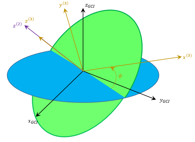
The final transformation matrix is one of the ingredients we were seeking as is given by
\[ {\mathcal A} = \left[ \begin{array}{ccc} \cos \phi \cos \psi – \sin \phi \sin \psi \cos \theta & \cos \phi \sin \psi \cos \theta + \sin \phi \cos \psi & \sin \psi \sin \theta \\ -\sin \phi \cos \psi \cos \theta – \cos \phi \sin \psi & \cos \phi \cos \psi \cos \theta – \sin \phi \sin \psi & \cos \psi \sin \theta \\ \sin \phi \sin \theta & -\cos \phi \sin \theta & \cos \theta \end{array}\right] \; . \]
Each of the Euler angles has an associated rate $$\left\{\dot \phi, \dot \theta, \dot \psi\right\}$$. The angular velocity in the body frame is related to these rates through
\[ \vec \omega = \vec \omega_{\phi} + \vec \omega_{\theta} + \vec \omega_{\psi} = \dot \phi \hat z_{GCI} + \dot \theta \hat x^{(1)} + \dot \psi \hat z^{(2)} \; .\]
The utility of pulling out the intermediate basis vectors should now be clear.
Carrying out the multiplication gives
\[ \vec \omega = \left[ \begin{array}{c} \dot \theta \cos \phi + \dot \psi \sin \phi \sin \theta \\ \dot \theta \sin \phi – \dot \psi \cos \phi \sin \theta \\ \dot \phi + \psi \cos \theta \end{array} \right]_{GCI} \; ,\]
which is the accepted answer (e.g. problem 19 in Chapter 4 of Goldstein).
The final step is to express this vector’s components in the body frame. This is done by multiplying the column array of inertial components by $${\mathcal A}$$ to get
\[ \vec \omega = \left[ \begin{array}{c} \dot \phi \sin \psi \sin \theta + \dot \theta \cos \psi \\ \dot \phi \cos \psi \sin \theta – \dot \theta \sin \psi \\ \dot \phi \cos \theta + \dot \psi \end{array} \right]_{Body} \; ,\]
which, again, can be favorably compared with Section 4-9 of Golstein (page 179 in the second edition).
The method outlined above is the most straightforward and pedagogically sound one I know. Admittedly, the multiplications and trigonometric simplifications are tedious but with a modern computer algebra system, such as wxMaxima, it can be readily done.